based on disturbance observer

(1)

https://doi.org/10.5194/ms-8-323-2017

Toward force detection of a cable-driven micromanipulator for a surgical robot

Wenjie Wang, Lingtao Yu, and Jing Yang

College of Mechanical and Electrical Engineering, Harbin Engineering University, Harbin, 150001, China Correspondence to: Lingtao Yu ([email protected])

Received: 9 May 2017 – Revised: 15 September 2017 – Accepted: 8 October 2017 – Published: 15 November 2017 Abstract. Force sensing plays an important role in minimally invasive surgery (MIS). Force sensing makes it possible for the surgeon to feel the tissue properties and apply an appropriate level force and avoid tissue damage.

The micromanipulators are compact and to allow appropriate disinfection, it is inappropriate to integrate sensors at the end of the micromanipulator. In this study, a new asymmetric cable-driven type of micromanipulator for a surgical robot was designed, and a joint angle estimator (JAE) was designed based on the dynamical model of the single cable-driven joint. Closed-loop control of the joint angle was carried out by regarding the JAE output as the feedback signal. On this basis, an external force estimator was designed using a disturbance observer (DOB).

The experimental results show an average accuracy of the joint angle estimator of about −0.150 ◦ , with excellent control precision, the largest absolute error of about 0.95 ◦ , and an average error of 0.175 ◦ . The accuracy of the force estimator was at a high level during static loading. The estimated accuracy was 94 % at external force is greater than 1 N, and the estimated accuracy was 82 % for an external force of 0.3 N. These results predict that force sensing of a cable-driven micromanipulator in this paper can used to realize the micromanipulator’s force feedback of a minimally invasive surgical robot.

1 Introduction

With the development of robot technology, robot-assisted surgery has been widely applied. ZEUS (Haidegger and Benyo, 2008) and the Da Vinci (Monsarrat et al., 2009) are the two most successful systems of a minimally invasive surgery robot (MISR). Most problems encountered during early clinical procedures have been solved. However, a major deficiency of MISR is the lack of force-sensing information feedback. The lack of this information may result in significant harm and trauma to normal tissue (Tholey et al., 2005).

It is difficult to apply accurate operating force to tissue dur- ing accurate operations, such as separation and suture. The force sensing for MISR systems is an active research sub- ject, as improved force sensing will improve surgical opera- tion skills and the quality of the procedure (Ortmaier et al., 2007). Specifically, force sensing improves the performance and efficiency of MISR systems by reducing the contact force

peak and decreasing the task execution time (Okamura et al., 2011).

The force estimation methods for MISR systems can be roughly divided into direct detection and indirect detection methods based on electric resistance or fiber and the displacement of the actuator input, respectively (Fu et al., 2014). Yin and Guo (2016) designed a teleoperated robot–

assisted catheter operating system with haptic. The sensors

for force sensing include strain gauge-based force sensors,

piezo-resistive force sensors, capacitive force sensors, piezo

magnetic force sensors, optical force sensors, vision-based

force sensors, and electroactive force sensors, among oth-

ers (Ma et al., 2014; Wei and Xu, 2015). Strain gauge is

the most commonly used force detecting element. In order

to realize the precise measurement of force, strain gauges

are typically put on the elastomer. If an external force is ap-

plied on the elastomer, the resistance of the strain gauge and

the electricity bridge voltage will be changed, so the exter-

nal force can be detected by measuring the changes in the

(2)

resistance bridge output voltage. Brown (2002) developed a motor driven grasping apparatus and measured the force and organizational characteristics using a strain gauge. It is important to reduce friction to improve the accuracy of force detection because the detecting element is far away from the point of interaction forces. Some researchers such as Mayer et al. (2008), Prasad et al. (2003), Kuebler et al. (2005) measured the instrument’s force directly using micro-force sensors installed in the manipulator’s end. Because the grating sensor has good magnetic resonance, Peirs (2004), and Puangmali et al. (2012) developed a three-dimensional force detection unit based on the use of grating. Lim (2014) realized the clamping force test by installing a grating sensor in the forceps of a micromanipulator. Xie (2015b) developed a new contact two-dimensional force sensor used in flexible micro devices based on optical fiber, with accuracy that can reach 83 %. Zhang et al. (2017) evaluated the performance of a strain-gauge force sensor for a haptic robot- assisted catheter operating system. Xu (2015) designed a novel compliant gripper with integrated position and grasping/interaction force sensing. Xie et al. (2016) researched the array platform for robotic cell microinjection force measurement. Conductive polymer materials can also be used to man- ufacture detecting elements. The researchers (Valdastri et al., 2006) of Verimetra Company has pursued microfabrication technology to design intelligent surgical instruments. They used the instrument itself as a substrate to create a semicon- ductor strain gauge, in which the strain gauge was embedded on the surface of the forceps or knives. However, this equip- ment has only been used in a small range, since the MISR instrument is a compact construction, and it is unsuitable to install sensors in the end of a manipulator because of the need for sterility. Additionally, surgical instruments are consum- able, thus increasing the operation cost.

One of the simplest ways to detect force is to detect the displacement changes of the elastic element. Rosen et al. (1999) designed a teleoperation endoscopic gripper with force feedback. Comparison of the position reference input and the actual position allows the generation of a position error when the gripper clamps human tissue and a clamping force will be automatically detected during operation. Friction and mechanical clearance can cause a position error, or a torque estimation error. Tholey (2004) realized indirect measurement of clamping force by detecting the motor current. The measurement error is big in this system due to the mechanism. Zhao (2015) realized the force estimate of micro device through a motor current, but the accuracy is too low when the external force is less than 2 N. Haraguchi (2016) developed a micro device with 4 DOFs and estimated the force information of the micro device using a neural network. Hong- bing Li (2013) realized the force testing of a 3 DOF micro instrument based on a disturbance observer, with a minimum resolution of 0.5 N.

In conclusion, the cost of direct force measuring is high and the limitations are obvious. The cost is low with good

Motor

Motor Motor Motor

Spring Joint

Joint Joint (a)

(b)

(c)

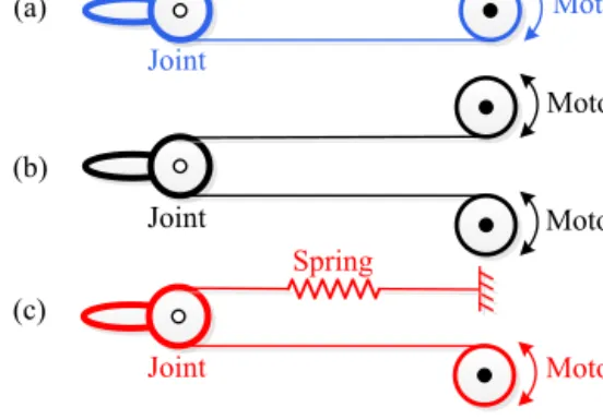
Figure 1. The three different basic cable-driven mechanisms.

adaptability if an integrated sensor in the end of the micro device driving mechanism is used to measure cable tension and estimate the external forces of the micromanipulator indi- rectly based on motion control and drive information. Over- all, indirect force detection can avoid several problems and the development of an indirect force detection method for the micromanipulator of a surgical robot based on a disturbance observer is the focus of this study.

The remainder of this paper is organized as follows. The cable-driven micromanipulator and the single joint principle prototype are described in Sect. 2. The dynamics, closed loop control of the finger angle based on the angle estimator and force detection method based on disturbance observer are proposed in Sect. 3, the experimental results of motion con- trol and force detection are shown in Sect. 4. Conclusions and future works are provided in Sects. 5 and 6, respectively.

2 The cable-driven micromanipulator and the single joint principle prototype

2.1 The cable-driven system mechanism

The torque generated by a motor is transmitted through a flexible cable in a cable-driven system. The force or torque in two different directions is required to drive a rotational joint, but the cable cannot transmit forces in the pushing direction. Three different basic cable-driven mechanisms have been used to satisfy these requirements, as shown in Fig. 1.

As shown in Fig. 1a, the mechanism can drive one joint with one motor. The structure is simple, so it is widely used in many robotic manipulators. However, sometimes it is difficult to ensure that the non-pulled side is tensioned, which will cause backlash and slow responses. This will seriously affect the performance of the mechanism, so it is essential to add a pre-tensioning mechanism, which will add to the com- plexity of the system.

In the second mechanism, shown in Fig. 1b, each cable

is independently driven by one motor. This mechanism pro-

vides high performance and it is easy to design the cable

routing structure. The joint stiffness can be easily adjusted

(3)

Griper A

axis

Gripper B

Gripper A

idler pulley spring motor Driven flexible rope

FM F^S

Ma

F

S

Fb Sa

F

M

Fb

axis A

3 ^M

Fr F^S^r

The wrist of the

micromanipulator axis

z

1p

z

3a

z

1p

z

2a

A

2

z

3a

z

3b

P itch joint

A

3 Griper B

Deflection joint

A

2

(a) (b)

A

1

The driving wheel of A

2

The 3 DOF micromanipulator

wrist

Figure 2. (a) Cable-driven mechanism of the micromanipulator. (b) The 3-D model of the micromanipulator wrist.

Cable tension Cable tension

Positive driving cable module

negative driving cable module

Positive driving cable Spring

DC servo motor

Grating ruler

component 1 Photo electric switch Grating ruler component 2

Micro magnetic encoder

gripper

Gripper module Negative

driving cable Fw2

Fw1

Figure 3. 3-D model of the single joint prototype.

by controlling the two motors. However, the cost is higher, as the number of required motors is doubled compared with other mechanisms, and application is limited by the require- ment of compact space.

As is shown in Fig. 1c, the third mechanism uses a spring for the reversed actuation of one side, and a motor is used to drive the other side. The cables can be tensioned by pulling the spring to an appropriate distance. This will apply two di- rectional forces to the joint. The cable tension can always be maintained without an additional pre-tensioning mechanism. Due to simple cable routing, the appropriate cost and the character of the tensioning itself makes the spring-motor mechanism a good choice when compact structures are required.

From the analysis above, the spring-motor mechanism (shown in Fig. 2c) was selected for the design of the micromanipulator.

2.2 The cable-driven micromanipulator for surgical robot The mechanism of the micromanipulator for a surgical robot is shown in Fig. 2a. The four different colours represent the

drive mechanism of different joints, with each joint designed based on the spring-motor mechanism. The micromanipula- tor has four DOFs, and the wrist of the micromanipulator has 3 DOFs, consisting of one pitch joint and two deflection joints. The driving force of each joint is determined by the difference between the tensions of the cables in each loop of the joint cable routing. The opening, closing, and deflection of the wrist are determined by the different combinations of the rotation directions of the motors used in gripper A and gripper B. The 3-D model of the wrist is shown in Fig. 2b.

The wrist and the driven components are driven by a rotary joint. The components of each joint are similar to those of the single joint prototype, as shown in Fig. 3.

2.3 The force analysis of the micromanipulator

The dynamic equation of operating forceps is shown in Eq. (1) and takes the external force of the system and the joint friction torque into consideration.

τ i = D i (q) ¨ q + H i (q, ˙ q) + G i (q) + τ f i + J T i F i ext . (1)

(4)

Part 6: negative driving cable model

K

m

i

m



m

J

m

B

_m ^m

i

r z



l

F

l

B

w1

m

1

y

1

K

w1

F

w1

x

1

r  J f

e

,

efc

, f

efv

, m l

e

,

g



F

ext

l

e

 z x

y



e

F

w2

y

2

m

0

x

2

B

w2

K

w2

m

2

K

sp

m

3

x

2

F

T20

Part 4:Spring

F

w1

F

w2

Part 5: guide-slider and idler component 2

Part 5: guide-slider and

idler component 2

f2

F

f1

F

Part 3: positive driving cable

Part 3: positive

driving cable

Part 2: guide-slider

and idler component 1

Part 2: guide-slider and idler component 1

Part 1：motor，Reducer

and rope wheel

Part 1：motor，Reducer

and rope wheel

Part 7: Gripper joint

Part 7: Gripper joint F

2

Figure 4. The mechanism model diagram of the single joint principle prototype.

Where i = a, b, a and b represent gripper A and gripper B respectively. τ i , D i (q), H i (q, ˙ q), G i (q), τ f i , J T i and F i ext are the joint driven torque, inertia matrix, centrifugal force and Coriolis force, gravity, friction torque, force Jacobian matrix and external force respectively. The driving torque of each joint is shown in Eq. (2); the meaning of the superscript i is similar to Eq. (1). Where, F M is the tension of the positive driven cable. F S is the tension of the negative driven cable.



 



 



τ 1 = r 1 F M r − F S r τ 2 = r 2 (F M − F S ) τ 3 i = r 3 F M i − F S i τ i = τ 1 τ 2 τ 3 i T

.

(2)

When the external force is zero, the micromanipulator moves freely. The dynamic equation of the operating forceps is shown in Eq. (3), and the parameters can be obtained by in- verse dynamics identification.

τ ˆ i = h

τ ˆ 1 τ ˆ 2 τ ˆ 3 i i T

= ˆ D i (q) ¨ q + ˆ H i (q, ˙ q) + ˆ G a (q) + ˆ τ f i . (3) When the external force is not equal to zero, the external force can be obtained from Eq. (4), where τ i is the actual joint torque and ˆ τ i is computed by the parameters in Eq. (3).

Digital filtering can be used first to obtain the data of τ i and τ ˆ i .

F i ext = J −T i τ i − ˆ τ i . (4)

The external force F ext applied on the micromanipulator and the clamping force F cp of the micromanipulator can be described as in Eq. (5).







F ext = F a ext + F b ext F cp = 1

2

F ext ya

+ F ext yb

. (5)

2.4 The prototype of the micromanipulator based on a single joint model

The four joints drive the micro devices and the cable routing structure as presented in the analysis above. The perfor-

mance of the single joint principle prototype can illustrate the performance of the micromanipulator. The prototype of the single joint model was designed as shown in Fig. 3. The DC servo motor provides the positive driving force and the re- turn spring provides the negative driving force. The displace- ments of the flexible cables were measured by two sets of raster detection modules and a non-contact micro magnetic encoder was used to detect the joint angle of the gripper. A photoelectric switch provides the origin signal of the system.

3 The force estimates research of the cable-driven micromanipulator prototype

3.1 The dynamic model and the joint angle estimator of the single joint prototype

The mechanism model diagram of single joint principle prototype is shown in Fig. 4. The model can be divided into six parts. Because the flexible cable moves at a low speed, high- frequency tremors are negligible, and the model of flexible cable is equivalent to a mass-spring-damper model. Motor movement cannot be completely passed to the slider. The displacement of slider 1 and the positive driving cable is determined by the detection value of grating ruler component 1, and the displacement of slider 2 and the negative driving cable is determined by the detection value of grating ruler component 2. The friction influence of the subsystems should be considered, and the gravitational effect of the gripper can be ignored since the gravity direction of the gripper direction and rotation direction are both vertical.

The dynamic equilibrium equations were established indi- vidually, as is shown below. When the system is in the orig- inal position, the flexible cables are in astatic state, and the joint angle and the displacement of sliders are zero. The relationship of the initial tensioning force of the positive driving cable and the negative driving cable are shown in Eq. (6), and F 0 is the initial tension of the system.

F w10 = F w20 = F 0 . (6)

(5)

ref

i

m

f

_d

  ' +

^dis

B

^m



m

1 J s

1

m

s

K 

dis mn

g J



dis dis

g s g 

dis mn

g J

dis m

ˆ

_d

ˆ ' + ˆ f   B 

Robot（motor）

DOB



dis1

Figure 5. The basic block diagram of DOB.

ref

i

m

1 m

+

m d

i

f F r B

z 



m

1 J s

1

m

s

K 

dis mn

g J



dis dis

g s g 

dis mn

g J

Robot（motor）

EFOB

1 m m

ˆ / + ˆ

d i

f   F r  z B 

e

1

l

_m

z r

i

r ˆ

ext

F  ˆ

ext

Figure 6. The external force estimator for the single joint system model based on DOB.

The model of part 1 is shown in Eq. (7), where, i m is the motor armature current, F 1 is the load of the rope wheel, τ l is the load torque, τ m is the input torque, z i is the reduction ratio, r m is the effective radius of the rope wheel, K m is the torque constant, J m is the effective moment of inertia of the DC motor, B m is the viscous damping constant, ¨ ϕ and ˙ ϕ are the angular acceleration and angular velocity of the motor, respectively.



 

 

τ m − τ l = J m ϕ + B ¨ m ϕ ˙ τ m = K m i m

τ l = r m

z i

F l .

(7)

The model of the guide-slider and the idler component 1 (part 2) is shown below, where F w1 is the cable tension that drives the gripper joint, m 0 is the mass of slider 1, ¨ x 1 is the slider acceleration,τ f 1 is the equivalent friction of part 2 and

Control software interface

Joint module

External force Fext

Motor servo driver

Grating module Spring Motor

Guide rail sliding block Driver module

Micro magnetic encoder

Inductor of the encoder Gripper Cable

Figure 7. Experimental design of the single joint prototype system.

is composed of viscous friction and coulomb friction, f sv1 and f sc1 are the coulomb friction coefficient and the viscous friction coefficient, respectively, sgn(·)is the symbolic func- tion, and ˙ x 1 is the slider velocity.

F 1 − F w1 = m 0 x ¨ 1 + τ f 1

τ f 1 = τ f 1

_sv

+ τ f 1

_sc

= f sv1 x ˙ 1 + f sc1 sgn ( ˙ x 1 ) . (8) As the mass of the positive driving cable is very small, the viscous friction coefficient B w = 2ξ w √

m 1 K w , and the influence of viscous friction and mass can be ignored to simplify the model. The model of the positive driving cable (part 3) can be regarded as a spring model, as is shown in Eq. (9).

K w is the elastic coefficient of the positive driving cable and y 1 is the displacement of one side of the positive driving cable, which is fixed to the gripper joint.

F w1 = K w1 (x 1 − y 1 ) + F w10 . (9)

The model of the spring (Sect. 4) is shown in Eq. (10). F 2 is the spring tension, K s is the elastic coefficient of the spring, and x 2 is the displacement of the spring mobile side.

F 2 = K s x 2 + F w20 . (10)

Similarly to part 2, the model of the guide-slider and idler component 2 (part 5) is shown in Eq. (9), and the variables in Eq. (11) are defined as in part 2.

F w2 − F 2 = m 0 x ¨ 2 + τ f 2

τ f 2 = τ f 2

_sv

+ τ f 2

_sc

= f sv2 x ˙ 2 + f sc2 sgn ( ˙ x 2 ) . (11) Similarly to part 4, the model of the negative driving cable (part 6) is shown in Eq. (12), and the variables in Eq. (12) are defined as in Eq. (9).

F w2 = K w2 (y 2 − x 2 ) + F w20 . (12)

(6)

im vi vp

K K



s Speed control

Km



^m



dis

P D

K



K s Position control



d

s



Position control mode

m

1

J s Bm



 



d

Kd

Figure 8. Control block diagram of the parameter identification for the joint angle estimator.

The dynamic model of the gripper joint (part 7) is shown in Eq. (13), where, θ , τ e , m e , J e and r are the gripper joint angle, joint driven torque, joint effective mass, joint equivalent moment of inertia, and the effective radius of the cable tension, respectively. τ ef is the friction torque of the joint and is composed of the viscous friction torque and the coulomb friction torque τ ext is the external force moment, and l e is the effective radius of the external force F ext .



 



 



τ e = J e θ + τ ¨ ef + τ ext

τ e = (F w1 − F w2 ) r

τ ef = τ efv + τ efc = f efv θ + f ˙ efc sgn( ˙ θ) τ ext = F ext l e .

(13)

The relationship between the joint angle θ and y 1 , y 2 is shown below, y 1 is the displacement of the positive driving cable which is fixed on the gripper, and y 2 is the displacement of the negative driving cable.

y 1 = y 2 = rθ. (14)

Combining Eqs. (6), (11), (12), and (14), the two different expressions of F w2 can be obtained, as shown below.

F w2 = K w2 rθ − K w2 x 2 + F 0

F w2 = m 1 x ¨ 2 + f sv2 x ˙ 2 + f sc2 sgn ( ˙ x 2 ) + K s x 2 + F 0 . (15) Then the relationship between x 2 and θ can be found as shown in Eq. (16). Equation (16) is the overall model of the joint angle estimator. The parameter identification and the practical application will be demonstrated in the experimen- tal section.

θ = m 1

K w2 r x ¨ 2 + f sv2

K w2 r x ˙ 2 + f sc2

K w2 r sgn( ˙ x 2 )+ K s + K w2

K w2 r x 2 . (16) 3.2 The force estimator of the single joint principle

prototype based on DOB

The DOB regards the difference between the actual output and the output of the dynamic model (without external force) as a disturbance applied on the system. When an external force is applied, the equivalent disturbance includes not only the modelling uncertainties but also the external force information. Therefore, force estimation based on the DOB must find the external force information from the equivalent disturbance. The advantage of the DOB is that it does not need force sensors or other sensors to estimate the external force.

The DOB is designed to achieve the external force detec- tion of the joint prototype system. The dynamics of a motor are described by the following equation.

J m ϕ = f ¨ d + K m i m ref

f d = τ 0 dis + B m ϕ. ˙ (17)

Where: J m , B m , ϕ, i m ref and K m denote the inertia mass, damping coefficient, position response, current, and the force coefficient of the motor, respectively. f d denotes the motor load, and is composed of damping and disturbance, and the disturbance includes the external force. The basic block diagram of the DOB is shown in Fig. 5, where J mn = J m , and g dis is the parameter of the low-pass first order filter s+g g

^dis

dis

. If τ dis1 = 0, the damping and disturbance are estimated using the low-pass first order filter as in the following equation.

f ˆ d = g dis

s + g dis f d . (18)

When the external force F ext is applied on the end of the gripper, the load of the rope wheel fixed on the motor is F 1 . If there is no external force applied on the end of the gripper, the load of the rope wheel fixed on the motor is F 1 0 and the relationship of F 1 and F 1 0 is as shown below.

F 1 = F 1 0 + F ext r. (19)

The external force estimator for the single joint principle prototype system is designed as shown in Fig. 6. The output of the external force estimator is shown below.

F ˆ ext = g dis

s + g dis

(f d − ˆ f d ). (20)

Where f d 0 = ˆ F 0 1 r m /z i + ˆ B m ϕ. To estimate the external force, ˙ the models of ˆ F 0 1 and ˆ B m must be known. The identification models of ˆ F 0 1 and ˆ B m are shown in the next part.

3.3 The identification models of ˆ B

_m

and ˆ F

₁

When the motor is running with no load,f d = B m ϕ, and ˙ τ dis1 = 0. The output of Fig. 5 is ˆ f d = ˆ B m ϕ, and Fig. 5 is the ˙ motor damping estimator. Parameter ˆ B m is a constant that can be obtained by the least square method.

When the single joint principle prototype system runs

without applied applied on the end of the gripper (F ext = 0),

let τ dis1 = ˆ B m ϕ, and f ˙ d = F 1 0 r m /z i + B m ϕ. Then, the output ˙

(7)

0 20 40 60 80 100 120 140 160 180 -50

0 50

Time (s)

Joint angle (°) Actual value

Identified value

0 20 40 60 80 100 120 140 160 180

-1 0 1

Error (°)

Time (s)

Figure 9. Identification result of the joint angle estimator model.

0 20 40 60 80 100 120 140 160 180

-50 0 50

Time (s)

Joint angle (°) _Desired

Actual

0 20 40 60 80 100 120 140 160 180

0 2 4

Time (s)

Error (°)

Figure 10. The performance of the control system without a joint angle estimator.

of disturbance observer in Fig. 5 is ˆ f d = ˆ F 0 1 r m /z i , and then F ˆ 0 can be determined by the equation below.

F ˆ 0 1 = ˆ f d z i /r m . (21)

When the external force F ext is applied on the end of the gripper, we must get the estimated value of F 1 0 from the information we obtain on the state of the gripper contacting the environment. If the system is running without the application of external force on the gripper (F ext = 0), the relationship of F 1 0 and F 1 is F 1 = F 0 1 . The three models of F 1 0 were established by dynamic analysis of the single joint prototype system.

Model A: the model is established based on the dynamics analysis of part 2 and part 3. Combined Eqs. (6), (8) and (9), the expression of F 1 0 is shown below.

F

₁⁰

= m

₀

x ¨

₁

+ f

_sv1

x ˙

₁

+ f

_sc1

sgn ( ˙ x

₁

) + K

w1

x

₁

− K

_w1

rθ + F

₀

. (22) Model B: the model is established based on the dynamic analysis of part 2, part 6, and part 7. Combining Eqs. (6), (8) and (12), (13) and (14), the expression of F 1 0 is shown

below.

F 1 0 = J e r

θ + ¨ f efv r

θ + ˙ f efc

r sgn( ˙ θ) + K w2 rθ + m 0 x ¨ 1 + f sv1 x ˙ 1 + f sc1 sgn ( ˙ x 1 ) + m 1 x ¨ 2 + f sv2 x ˙ 2

+ f sc2 sgn ( ˙ x 2 ) − K w2 x 2 + F 0 . (23) Model C: the model is established based on the dynamic analysis of parts 2, 4, 5 and 7. Combining Eqs. (6), (8), (10), (11), (13) and (14), the expression of F 1 0 is shown in Eq. (24).

F

₁⁰

= J

_e

r

θ + ¨ f

_efv

r

θ + ˙ f

_efc

r sgn( ˙ θ) + m

0

x ¨

₁

+ f

_sv1

x ˙

₁

+ f

_sc1

sgn ( ˙ x

₁

) + m

₁

x ¨

₂

+ f

_sv2

x ˙

₂

+ f

_sc2

sgn( ˙ x

₂

) + K

s

x

₂

+ F

₀

. (24) The actual value of F 1 0 and f d can be determined by the output of Fig. 5, as shown in the analysis above. The identification experiment and identified value of the model parameters are described in the next section.

4 Experimental research

The experimental system is shown in Fig. 7, and the specifi- cations are listed in Table 1. Encoder information acquisition of the motion control card (Leisai DMC2610) was used to ac- quire the displacements of grating scales and the angle of the gripper. The driving force arm of the gripper joint is 4 mm, and the length of the gripper is 20 mm. The external force was applied by loading weights, using Labview software and a Microsoft windows XP operating system.

4.1 Parameter identification and the performance of the joint angle estimator

In order to identify the parameters of the joint angle estimator, a micro magnetic encoder was used to detect the actual angle of only the gripper joint. The micro magnetic encoder has no effect on the control. The angle of the motor was used as the feedback signal. In other words, the motor was un- der closed-loop control, but the gripper joint angle was controlled by open-loop control, as shown in Fig. 8. The gripper angle θ can be obtained through the micro magnetic encoder, and x 2 can be obtained using the grating ruler. Then, the parameters of the joint angle estimator model can be identified by the least squares method. The identification model is shown below. The meaning of the parameters ρ s in Eq. (25) is the error vector.

Y s = W s χ s + ρ s (25)







Y s = θ,W s = ¨ x 2 x ˙ 2 sgn( ˙ x 2 ) x 2 χ s =

m 1 K w2 r

f sv2 K w2 r

f sc2 K w2 r

K s + K w2 K w2 r

T

. (26)

Where, x 2 is the position detected value of the Grating ruler

component 2, ˙ x 2 is the speed, and ¨ x 2 is the acceleration, and

sgn( ˙ x 2 ) is the symbolic function.

(8)

264.4277 3.1606

im vi vp

K K



s Speed control

Km ^m



dis

P1 D1

K



K s Position control



d

s



 ˆ

x2

Speed control mode

m

1

J s Bm



s

Joint angle estimator



s 0.008

sgn( )

0.0025

Figure 11. The control block diagram with a joint angle estimator.

Table 1. Specifications of the experiment system.

Specifications

Motor Maxon RE25 20 W, incremental

photoelectric encoder: 1000p/r, Reduction ratio 35 : 1

Servo drive Copley ACI-055-18

Grating reading head Renishaw :RH100X30D05A Resolution: 0.001 mm

Grating ruler RGS-40

Micro magnetic encoder reading head Renishaw :RM08ID0012B02L2G00(4096 p/r) Resolution: 0.001 mm

Micro magnetic encoder magnetic bead RMM44A3A00

Guide rail and slider MISUMI SSEBZ8L-85

Spring KSSC2189 0.6566 N mm −1

0 20 40 60 80 100 120 140 160 180 200

-50 0 50

Time (s)

Joint angle (°) Desired

Actual Estimation

0 20 40 60 80 100 120 140 160 180 200

-1 0 1

Time (s)

Error (°)

Error 1 Error 2

Figure 12. The performance the control block diagram with a joint angle estimator.

Through the identification experiment, the parameters vector can be determined, as shown below.

χ ˆ s = [0.0805 0.5225 0.0025 264.3560] T .

The actual data, the identification result of the joint angle, and the errors are shown in Fig. 9. The average of the iden- tification error is 0.2750 ◦ the maximum identification error

0 20 40 60 80 100 120 140 160

-50 0 50

Time (s)

Joint angle (°) Desired Actual Estimation

0 20 40 60 80 100 120 140 160

-1 -0.5 0 0.5 1

Time (s)

Error (°)

Tracking error Estimation error

Figure 13. The test results of the robustness of the control system.

is 0.8355 ◦ , and the minimum of the identification error is

− 0.8321 ◦ . These values indicate good accuracy of the joint angle estimator.

The performance of the general control system is shown

in Fig. 10. There was significant error between the desired

trajectory and the actual trajectory. The average error was

(9)

0 5 10 15 20 25 30 -200

0 200

Time (s)

Motor angle (rad)

0 5 10 15 20 25 30

-0.01 0 0.01

Time (s)

Motor torque (N m)

Experimental Identification

Figure 14. The identification experimental result of motor viscous damping.

0 5 10 15 20 25 30

-200 0 200

Time (s)

Motor angle (rad)

0 5 10 15 20 25 30

-0.01 0 0.01

Time (s)

Motor torque (N m)

Experimental Verification

Figure 15. The verification experimental result of motor viscous damping.

1.912 ◦ , the maximum error was 4.134 ◦ , and the minimum was 0.964 ◦ . The performance does not the requirements for micro devices of precise operation.

In order to verify the performance of the joint angle estimator, a control system was designed and is shown in Fig. 11.

The output of the joint angle estimator is the feedback signal of the position loop, the position control is a PD control and the speed control is a PI control. The parameters can be set through the servo drive. The parameters of the controller are shown below.

Position loop : K p1 K D1 = [98 14]

Speedloop : K vp K vi = [100 40] .

The desired trajectory and the actual trajectory are shown in Fig. 12. When the gripper joint is driving with no external force, the desired trajectory, the actual trajectory, and the estimated trajectory are almost the same. The average error between the desired trajectory and the actual trajectory was −0.150 ◦ , the maximum error was 0.905 ◦ , and the minimum error was −0.974 ◦ . The average error between the actual trajectory and the estimated trajectory was 0.170 ◦ , the maximum error was 0.715 ◦ , and the minimum was −0.498 ◦ . Overall, the control precision of the system is higher than the

0 20 40 60 80 100 120 140 160 180 200

-50 0 50

Time (s)

Joint angle (°)

0 20 40 60 80 100 120 140 160 180 200

10 20 30

Time (s)

Rope tension Fl (N)

0 20 40 60 80 100 120 140 160 180 200

-10 0 10

Time (s)

Rope tension Fl error (N)

Actual Model A Model B Model C

Model A error Model B error Model C error

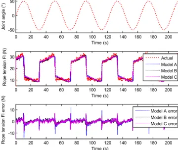
Figure 16. The identification results and the identification errors of the three models.

0 20 40 60 80 100 120 140 160 180 200

-50 0 50

Time (s)

Joint angle (°)

0 20 40 60 80 100 120 140 160 180 200

10 20 30

Time (s)

Rope tension Fl (N)

Experimental Identification

Figure 17. The identification result of the simplified model C.

system without a joint angle estimator. In other words, the joint angle estimator works well and the necessary precision can be obtained.

To test the robustness of the control system, a complex tra-

jectory was used to assess the performance of the control sys-

tem and the joint angle estimator when an external force of

2.5 N was applied on the gripper. The experimental result is

shown in Fig. 13. The average error between the desired tra-

jectory and the actual trajectory is −0.105 ◦ . The maximum

error is 1.202 ◦ , and the minimum is −1.271 ◦ . The average er-

ror between the actual trajectory and the estimated trajectory

is 0.076 ◦ , the maximum error is 0.508 ◦ , and the minimum

error is −0.454 ◦ . These values indicted excellent robustness

of the control system and the joint angle estimator.

(10)

0 20 40 60 80 100 120 140 160 -50

0 50

Time (s)

Joint angle (°)

0 20 40 60 80 100 120 140 160

10 20 30

Time (s)

Rope tension Fl (N)

0 20 40 60 80 100 120 140 160

-10 0 10

Time (s)

Tension Fl error (N)

Experimental Verification

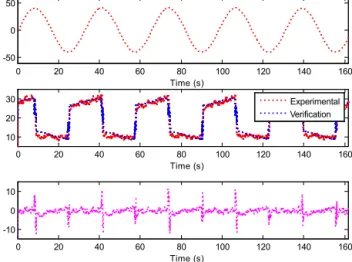
Figure 18. The verification result of the simplified model C.

Fext

Weights Fext

Weights 0°

Fext

Weights 30°

Weights

-40°

Fext

Weights

Weights Fext

Figure 19. External force estimation experimental system.

4.2 The identification experiment of ˆ B

_m

and ˆ F

⁰₁

The motor was controlled without applied load on the motor output shaft, so that the actual output torque ˆ f d can be obtained according to Fig. 5, and ˙ ϕ can be obtained from the motor encoder. The relationship between ˆ f d and ˙ ϕ is f ˆ d = B m ϕ ˙ can be determined and then the parameter B m can be calculated by the least square method. The identification value of B m is 1.6934 × 10 −5 Nm rad −1 . The identification experimental result is shown in Fig.14, and the verification experimental result is shown in Fig. 15. The result shows good precision of the identification of motor viscous damping.

The identification experiment was performed based on the joint angle closed-loop control by regarding the joint angle estimator output as the feedback signal. The control block diagram is shown in Fig. 11. The actual value of F 0 1 can be obtained as described in the analysis in Sect. 3.3. The values of the observation matrixes can be obtained by reading the grating sensors and the micro magnetic encoder. The three different models of F 0 1 are shown in Sect. 3.3, where the model C can be represented by the following expression,

0 10 20 30 40 50 60 70 80 90 100 110

-2 -1 0 1

Time (s)

Joint angle (°)

0 10 20 30 40 50 60 70 80 90 100 110

-3 -2 -1 0 1

Time (s)

Estimated force (N) -30 g -50 g -100 g -200 g -250 g

-30 g Desired -50 g -100 g -200 g -250 g

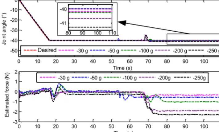
Figure 20. Negative direction loading experiment results at 0 ◦ .

1

0 10 20 30 40 50 60 70 80 90 100

-2 -1 0 1

Time (s)

Joint angle (°)

0 10 20 30 40 50 60 70 80 90 100

-1 0 1 2 3 4

Time (s)

Estimated force (N) 30 g 50 g 100 g 200 g 250 g

desired 30 g 50 g 100 g 200 g 250 g

Figure 21. Positive direction loading experiment results at 0 ◦ .

where x 1 is the position detected value of the grating ruler component 1, ¨ x 1 , ˙ x 1 and sgn( ˙ x 1 ) are acceleration, speed and symbolic function, respectively. The other models can similarly be written as expressions. The parameter matrixes of the three models can be obtained, and the identification results and the identification errors are shown in Fig. 16.

Y c = W c χ c + ρ c (27)



 



 

 Y c = ˆ

F 0 L

W c = θ ˙ ¨ θ sgn( ˙ θ ) ¨ x 1 x ˙ 1 sgn ( ˙ x 1 ) ¨ x 2 x ˙ 2 sgn( ˙ x 2 ) x 2 1 χ c = J e /r f efv /r f efc /r m 0 f sv1

f sc1 m 1 f vp2 f cp2 K s F 0 T .

The cable tension F 0 1 will have a larger error when the joint velocity is zero because the system has a hysteresis effect. The movement of the motor cannot be passed to the gripper immediately as the cable is not a rigid body.

When the joint velocity is non-zero the identification results are trustworthy. The average errors of the three models are

− 0.0228, 0.0189, and −0.0063 N respectively. The identifi-

cation precision of model C is higher than that of the others,

(11)

extF

0 20 40 60 80 100

-2 -1 0 1

0 20 40 60 80 100

0 2 4

0 20 40 60 80 100

0 20 40

0 20 40 60 80 100

-3 -2 -1 0 1

extF

①

②

③ ①

②

③ ④ ⑤

Time (s)

(a) Time (s)

(b)

(°) (°)

(N) (N)

Figure 22. The partition of the experimental results curve.

0 10 20 30 40 50 60 70 80 90 100 110

0 10 20 30 40

Time (s)

Joint angle (°)

0 10 20 30 40 50 60 70 80 90 100 110

-3 -2 -1 0 1

Time (s)

Estimated force (N)

-30g -50g -100g -200g -250g

-30 g -50 g -100 g -200 g 250 g

90 100 110

29 30 Desired

Figure 23. Negative direction loading experiment results at 30 ◦ .

so model C was adopted for further studies. The parameters and their standard variance are shown below.

χ ˆ

_c

= ˆ χ

_c1

χ ˆ

_c2

χ ˆ

_c3

χ ˆ

_c4

χ ˆ

_c5

χ ˆ

_c6

χ ˆ

_c7

χ ˆ

_c8

χ ˆ

_c9

χ ˆ

_c10

χ ˆ

_c11

T

= [0.1975 − 9.808 0.005 − 38.64 6705 3.259 38.99

− 4404 5.436 669.0 19.53]

^T

%σ

χ cˆ

= [32.29 % 27.3 % 2625 % 59.23 % 7.678 % 3.809 % 54.14 % 15.26 % 2.518 % 1.932 % 0.115 %] .

As the velocity and acceleration of the system are small and the standard variance ofχ c1 , χ c2 , χ c3 , χ c4 , χ c5 , χ c7 and χ c8 are over 5 %, so the influence of these parameters can be ig- nored. The simplified model C is shown below.

Y p = W p χ p + ρ p , (28)



 

 

Y p = ˆ F 0 L

W p = sgn( ˙x 1 ) sgn( ˙ x 2 ) x 2 1 χ p = f sc1 f cp2 K s F 0 T

.

(29)

The parameters of the simplified model C can be obtained through the LS method. The identification result of the simplified model C is shown in Fig. 17, and the values of the parameters and their standard variance are shown below. Another experiment was used to verify the simplified model C, as shown in Fig. 18. The average error was 0.011 N.

The above analysis illustrated the accuracy of the simplified

0 10 20 30 40 50 60 70 80 90 100 110

0 10 20 30 40

Time (s)

Joint angle (°)

0 10 20 30 40 50 60 70 80 90 100 110

-2 0 2 4

Time (s)

Estimated force (N)

30 g 50 g 100 g 200 g 250 g

85 90 95 100 29

30 31 Desired

Figure 24. Positive direction loading experiment results at 30 ◦ .

0 10 20 30 40 50 60 70 80 90 100 110

-50 -40 -30 -20 -10 0

Time (s)

Joint angle (°)

0 10 20 30 40 50 60 70 80 90 100 110

-3 -2 -1 0 1 2

Time (s)

Estimated force (N)

-30 g -50 g -100 g -200 g -250 g

-30 g -50 g -100 g -200g -250g

80 90 100 110 -41

-40

Desired

Figure 25. Positive direction loading experiment results at −40 ◦ .

model, suggesting the model can be used to estimate the external force applied on the gripper by the method presented in Fig. 6.

χ ˆ p = [3.879 5.027 707.7 19.52] T

%σ χ ˆ

c

= [3.025 % 2.658 % 1.787 % 0.115 %] . 4.3 The external force estimation experiment

The external force estimation strategy is shown in Fig. 6 in which the gripper was controlled by the method shown in Fig. 11. f d 0 = ˆ F 0 1 r m /z i + ˆ B m ϕ ˙ can be determined using the identification models in Sect. 4.1. External force applied on the gripper is shown in Fig. 19. The external force estima- tion experiments were performed by applying external forces on the gripper of different magnitudes and in different direc- tions. The positive direction and negative direction external forces were applied at 0, 30 and −40 ◦ , and external forces of 30, 50, 100, 200, and 250 g were tested. The experiment results are shown in Figs. 20 to 26.

The experimental results for a joint angle of 0 ◦ are shown

in Figs. 20 and 21. Fig. 22a shows the experimental process

when the external force is 2 N: (1) is the no-load region, (2) is

the loading process, and (3) is the stable region. The no-load

(12)

0 10 20 30 40 50 60 70 80 90 100 110 -40

-20 0

Time (s)

Joint angle (°)

0 10 20 30 40 50 60 70 80 90 100 110

-1 0 1 2 3 4

Time (s)

30 g 50 g 100 g 200 g 250 g

90 100 110

-40 -39 -38

Desired

Estimated force (N)

Figure 26. Positive direction loading experiment results at −40 ◦ .

error range of the external forces estimation is about ±0.1 N, with high accuracy of the force estimator. The estimated accuracy can reach up to 94 % for an external force greater than 1 N, and the estimated accuracy can reach 82 % for an external force of 0.3 N. The external force has little influence on the joint angle control precision. The greatest error was 1.25 ◦ for an external force of 2.5 N.

An experimental process is shown in Fig. 22b for a joint angle of 30 and −40 ◦ : (1) is the moving process, (2) is the adjustment process, (3) is the no-load region, (4) is the loading process, and (5) is the stable region. The dynamic no- load error is about ±0.15 N when external forces are applied on the positive direction. The dynamic no-load error is about

± 0.2 N when external forces are applied on the negative direction. The static no-load error is about ±0.15 N, with good accuracy of the force estimator. The estimated accuracy can reach 95 % when the external force is more than 1 N, and the estimated accuracy can reach 84 % when the external force is 0.3 N. The external force has little influence on joint angle control precision. The greatest error was 1.4 ◦ , when external force was applied to the gripper.

5 Conclusions

A new asymmetric cable-driven type of micromanipulator for surgical robot was described. Using a single joint sam- ple machine to verify the validity of the method proposed in this paper, a joint angle estimator was designed (JAE) based on the dynamical model of the single cable-driven joint. The average accuracy of the joint angle estimator was measured at about 0.2750 ◦ , with a maximum error of 0.8355 ◦ . The closed-loop control problem of the joint angle was solved by considering the joint angle estimator output as the feedback signal. The biggest tracking error was measured at about

± 0.9 ◦ . We designed the external force estimator using the method of disturbance observer, and the model parameters were identified and external force estimation experiments were performed. The experimental results shown that the static no-load error was about ±0.1 N and the dynamic load-

ing error was about ±0.15 N. The precision of the external force estimator can reach up to 94 % when the external force is more than 1 N, and the precision can reach 84 % at an external force of 0.3 N. In summary, the external force estimation method presented in this paper is effective and accurate, and can be used to realize force feedback for a minimally invasive surgical robot.

We will aim at realizing the external force estimation of the 4 DOFs micro device. Additionally, the hybrid control of position and force will be researched and let the surgeon feel the external force.

Data availability. All the data for this paper are given in the form of and figures, and can be obtained by requesting from the corre- sponding author.

Competing interests. The authors declare that they have no con- flict of interest.

Acknowledgements. This work partially supported by the National Natural Science Foundation of China (grant 61203358/F0306), the Natural Science Foundation of Hei- longjiang Province (grant F2015034), The central university basic scientific research business expenses project (HEUCFM170703).

We also greatly appreciate the efforts and helpful suggestions of the reviewers and our colleagues.

Edited by: Guangbo Hao

Reviewed by: three anonymous referees

References

Brown, J., Rosen, J., Moreyra, M., Sinanan, M., and Han- naford, B.: Computer-controlled motorized endoscopic grasper for in vivo measurement of soft tissue biomechanical characteristics. Medicine Meets Virtual Reality 02/10: Digital Upgrades, Applying Moore’s Law to Health, 85, 71–73, https://doi.org/10.3233/978-1-60750-929-5-71, 2002.

Fu, Y., Li, K., Pan, B., Zhan, J., and Wang, S: A Survey of Force Sensing and Force Feedback Technology for Robot- assisted Minimally Invasive Surgical System, Robot, 36, 117–

128, https://doi.org/10.3724/SP.J.1218.2014.00117, 2014.

Haidegger, T. and Benyo, Z.: Surgical robotic support for long duration space missions, Acta Astronautica, 63, 996–1005, https://doi.org/10.1016/j.actaastro.2008.01.005, 2008.

Haraguchi, D., Kanno, T., Tadano, K., and Kawashima, K.: A pneumatically driven surgical manipulator with a flexible distal joint capable of force sensing, IEEE-ASME Trans. Mechatron., 20, 2950–2961, https://doi.org/10.1109/TMECH.2015.2415838, 2016.

Kuebler, B., Seibold, U., and Hirzinger, G.: Development of ac-

tuated and sensor integrated forceps for minimally invasive

surgery, Int. J. Med. Robot. Comput. Assist. Surg., 1, 96–107,

https://doi.org/10.1002/rcs.33, 2005.

(13)

Li, H., Kawashima, K., Tadano, K., Ganguly, S., and Nakano, S.:

Achieving haptic perception in forceps’ manipulator using pneu- matic artificial muscle, IEEE-ASME Trans. Mechatron., 18, 74–

85, https://doi.org/10.1109/TMECH.2011.2163415, 2013.

Lim, S. C, Lee, H. K., and Park, J.: Grip force measurement of for- ceps with fibre Bragg grating sensors, Electron. Lett., 50, 733–

735, https://doi.org/10.1049/el.2013.4182, 2014.

Ma, C. Z., Du, J. S., Liu, Y. Y., and Chu, Y. K.: Overview of Micro- Force Sensing Methods, Appl. Mech. Mat., 462–463, 25–31, https://doi.org/10.4028/www.scientific.net/AMM.462-463.25, 2014.

Mayer, H., Gomez, F., Wierstra, D., Nagy,I.?Knoll, A., and Schmid- huber, J.: A system for robotic heart surgery that learns to tie knots using recurrent neural networks, Adv. Robot., 22, 1521–

1537, https://doi.org/10.1163/156855308X360604, 2008.

Monsarrat, N., Collinet, P., Narducci, F., Leblanc, E., and Vinatier, D.: Robotic assistance in gynaecological surgery:

state-of-the-art, Gynecol. Obstet. Fertil., 37, 415–424, https://doi.org/10.1016/j.gyobfe.2009.03.023, 2009.

Okamura, A., Verner, L., Reiley, C., and Mahvash, M.:

Haptics for robot-assisted minimally invasive surgery.

Robotics research, Springer Berlin Heidelberg, 66, 361–372, https://doi.org/10.1007/978-3-642-14743-2_30, 2011.

Ortmaier, T., Deml, B., Kuebler, B., Passig, G., Reintsema, D., and Seibold, U.: Robot assisted force feedback surgery, STAR, Springer Berlin Heidelberg, 31, 361–371, https://doi.org/10.1007/978-3-540-71364-7_22, 2007.

Peirs, J., Clijnen, J., Reynaerts, D., Brussel, H., Herijgers, P., Corteville, B., and Boone, S.: A micro optical force sensor for force feedback during minimally invasive robotic surgery, Sensor. Actuat. A-Phys., 115, 447–455, https://doi.org/10.1016/j.sna.2004.04.057, 2004.

Prasad, S., Kitagawa, M., Fischer, G., Zand, J., Talamini, M., Taylor, R., and Okamura, A.: A modular 2-DOF force-sensing instrument for laparoscopic surgery, Lect. Notes Comput. Sc., 2878, 279–286, https://doi.org/10.1007/978-3-540-39899-8_35, 2003.

Puangmali, P., Liu, H., Seneviratne, L., and Althoefer, K.: Minia- ture 3-axis distal force sensor for minimally invasive surgical palpation, IEEE-ASME Trans. Mechatron., 17, 646–656, https://doi.org/10.1109/TMECH.2011.2116033, 2012.

Rosen, J., Hannaford, B., MacFarlane, M., and Sinanan, M.: Force controlled and teleoperated endoscopic grasper for minimally invasive surgery – experimental performance evaluation, IEEE Trans. Biomed. Eng., 46, 1212–1221, https://doi.org/10.1109/10.790498, 1999.

Tholey, G., Pillarisetti, A., Green, W., and Desai, J.: Design, development, and testing of an automated laparoscopic grasper with 3-D force measurement capability, Proceedings of the In- ternational Symposium on Medical Simulation, Berlin, Ger- many: Springer-Verlag, 38–48, https://doi.org/10.1007/978-3- 540-25968-8_5, 2004.

Tholey, G., Desai, J., and Castellanos, A.: Force feed- back plays a significant role in minimally invasive surgery: Results and analysis, Ann. Surg., 241, 102–109, https://doi.org/10.1097/01.sla.0000149301.60553.1e, 2005.

Valdastri, P., Harada, K., Menciassi, A., Beccai, L., Ste- fanini, C., Fujie, M., and Dario, P.: Integration of a minia- turized triaxial force sensor in a minimally invasive surgical tool, IEEE Trans. Biomed. Eng., 53, 2397–2400, https://doi.org/10.1109/TBME.2006.883618, 2006.

Wei, Y. and Xu, Q.: An overview of micro-force sensing techniques, Sens. Act. A Phys., 234, 359–374, https://doi.org/10.1016/j.sna.2015.09.028, 2015.

Xie, H., Liu, H., Noh, Y.,Li, J., Wang, S., and Althoe- fer, K.: A fiber-optics-based body contact sensor for a flexible manipulator, IEEE Sens. J., 15, 3543–3550, https://doi.org/10.1109/JSEN.2015.2392384, 2015.

Xie, Y., Zhou, Y., Lin, Y., Wang, L., and Xi, W.: Development of a Microforce Sensor and Its Array Platform for Robotic Cell Microinjection Force Measurement, Sensors, 16, p. 483, https://doi.org/10.3390/s16040483, 2016.

Xu, Q.: Design and Development of a Novel Compliant Gripper with Integrated Position and Grasping/Interaction Force Sensing, IEEE T. Autom. Sci. Eng., 99, 1–14, https://doi.org/10.1109/TASE.2015.2469108, 2015.

Yin, X., Guo, S., Hirata, H., and Ishihara, H.: Design and experimental evaluation of a teleoperated haptic robot–assisted catheter operating system, J. Intell. Mater. Syst. Struct., 27, 3–

16, https://doi.org/10.1177/1045389X14556167, 2016.

Zhang, L., Guo, S., Yu, H., and Song, Y.: Performance evaluation of a strain-gauge force sensor for a haptic robot-assisted catheter operating system, Microsyst. Technol., 23, 5041–5050, https://doi.org/10.1007/s00542-017-3380-2, 2017.

Zhao, B. and Nelson, C. A.: Sensorless Force Estimation for a Three