Abstract—In recent years, the process of cellular
manufacturing and group technology has received much attention and popularity in many developed countries. By applying Group Technology (GT), many benefits of flow-line production can be attained in a batch production system. GT can improve material handling, significantly reduce material flow time and distance, and setup times. In this paper, a two step approach is proposed to solve the GT problem using Genetic Algorithms (GA). The first step assigns parts to the best available machines according to their required specifications. The second step forms manufacturing cells and part families. The proposed GA model has the flexibility of choosing the number of cells required, which is very useful in examining different manufacturing cell configurations; or in case that the workshop or factory prefers a certain number of cells. For example if the workshop or factory doesn't have the workspace required for more than four cells. To compare the performance of the proposed GA model, five part-machine matrices are obtained from the literature are solved using different techniques and their results are compared to the results achieved by the proposed GA model. The GA model results were found satisfactory and superior to other techniques in some cases.
Index Terms— Cellular Manufacturing, Genetic Algorithms,
Group Technology, Part-machine Matrix.
I. INTRODUCTION
Group technology is a manufacturing philosophy in which similar parts are identified and grouped together to take advantage of their similarities in manufacturing and design. Similar parts are arranged into part families. For example, a plant producing 10,000 different part numbers may be able to group the vast majority of these parts into 50 or 60 distinct families.
The objectives of Group Technology are best achieved in business concerned with small to medium batch production; these represent a major part of manufacturing industry. The traditional approach to this type of manufacturing is to make
Manuscript received January 7, 2008.
Hatim H. Sharif is a Master’s Student at the Department of Industrial and Management Engineering, College of Engineering and Technology, Arab Academy for Science and Technology, Abu Keer Campus, P.O. Box 1029, Alexandria, Egypt (e-mail: [email protected]).
Khaled S. El-Kilany, is an Assistant Professor at the Department of Industrial and Management Engineering, College of Engineering and Technology, Arab Academy for Science and Technology, Abu Keer Campus, P.O. Box 1029, Alexandria, Egypt (e-mail: [email protected]).
Mostafa A. Helaly is a Visiting Professor at the Department of Industrial and Management Engineering, College of Engineering and Technology, Arab Academy for Science and Technology on leave from Production Engineering Department, Faculty of Engineering, Alexandria University, Egypt (e-mail: [email protected]).
use of a functional layout in the factory, i.e. similar machines are grouped according to type. As a result of this form of machine layout, where only machining operations of a particular type may be performed in a limited area of the workshop, the work-piece itself must travel a considerable distance around the workshop before all the operations are performed upon it. This usually leads to a long throughput time. The planning of process route becomes an extremely difficult task since a number of similar machine tools may be considered at each point in the sequence of manufacturing operations.
Also, the scheduling and control in such a system are difficult because numerous alternatives are available. As a result, a different concept of manufacturing organization and layout has been developed to overcome these difficulties. This is the Group Technology (GT) concept whose emphasis lies in reducing the dimension of the situation to be controlled. Instead of being functionally laid out, the factory is divided into smaller cells in such a way that each cell is equipped with all the machines and equipment needed to complete a particular family of components. Each family would possess similar design and/or manufacturing char-acteristics. Hence, the processing of each member of a given family would be similar, and this results in better manufacturing efficiencies than the traditional manufacturing approaches [1, 2].
It has been found that by switching to this type of cellular manufacture, many benefits of flow-line production can be attained in a batch production system. The application of GT to a traditional manufacturing system can usually result in a simpler material flow system, so that a higher transfer rate and easier production planning and control functions can usually be achieved. This paper will present a genetic algorithm approach to the group technology problem.
Based on a set of part required design and manufacturing characteristics and a set of machine capabilities, the approach first selects the best machines to process the parts and then forms machine cells and part families. Thus, the GT problem is solved on two consecutive steps using two GA-based models.
The paper first defines the group technology problem and classifies the different approaches, presented by the literature, to solve this problem. Then a brief description of genetic algorithms is presented with a focus on the logic structure of GA. Afterwards, a detailed description of the developed models is given. Also, a comparison of the results obtained from the model to results of other techniques found in the literature is shown. Finally, the conclusions and remarks are pointed out.
A Genetic Algorithm Approach to the Group
Technology Problem
II. APPROACHES TO GROUP TECHNOLOGY PROBLEM
The biggest obstacle in changing over to group technology from a traditional production shop is the problem of grouping parts and machines into families.
There are many approaches to this problem [3-8]. These approaches are divided into two categories, which are the classical and the modern approaches (Fig. 1). This paper presents a new approach to solve the GT problem using Genetic Algorithms.
Approaches to Cellular Manufacturing
Classical Approaches
Modern Approaches
Visual Inspection
Classification and Coding
Systems
Product Flow Analysis
Artificial Neural Networks Fuzzy Models
[image:2.595.46.290.178.245.2]Genetic Algorithms Other
Fig. 1: Approaches to the Group technology Problem.
III. GENETIC ALGORITHMS
Genetic algorithms (GA) were formally introduced by John Holland in 1975 and have been applied in a number of fields, e.g. mathematics, engineering, biology, and social science. Genetic algorithms are search algorithms based on the mechanics of natural selection and natural genetics. They combine the concept of survival of the fittest with structured, yet randomized, information exchange to form robust search algorithms. The concept of GA mimics the evolution process that occurs in natural biology.
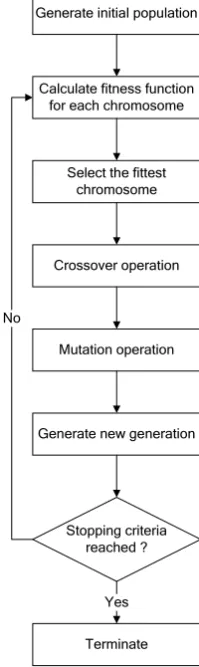
The logic structure behind the process of genetic algorithms process can be represented by the flowchart shown in Fig. 2.
Generate initial population
Calculate fitness function for each chromosome
Select the fittest chromosome
Crossover operation
Mutation operation
Stopping criteria reached ? Generate new generation
Terminate Yes No
Fig. 2: Logic Structure of Genetic Algorithms.
An initial population of possible solutions (referred to as individuals or chromosomes) is generated. The genetic pool of a given population potentially contains the solution, or a better solution, to a given adaptive problem. This solution is not "active" because the genetic combination on which it relies is split between several subjects. Only the association of different genomes can lead to the solution. The
chromosomes evolve through successive iterations, called
generations. During each generation, the chromosomes are evaluated using a measure of fitness.
To create the next generation, new chromosomes (offspring) are formed using crossover and mutation
operators. A new generation is formed by selection among the fittest chromosomes. Fitter chromosomes have higher probability of being selected. After several generations, the algorithm reaches stopping criteria and converges to the best chromosome, which represents the best found solution to the problem.
IV. PROPOSED GA MODEL DESCRIPTION AND MECHANISMS
To solve the GA problem, a two step procedure is used. To solve the GT problem, a two steps procedure is used. The first step is to select the best machine(s) for each part. The second step is to group the machines and parts into different number of sets (groups).
Machines and parts specifications defined by the user are the inputs for step one. The output of step one is the machines required for each part, which is then converted to un-clustered part-machine matrix.
This un-clustered part-machine matrix is now the input to step two. The function of step two is to cluster this un-clustered part-machine matrix. Based on the formed clusters, machine cells and part families are identified, which is step two output. Fig. 3 shows the inputs and outputs of the proposed method solution procedure.
The genetic algorithm models for the two steps where developed using Microsoft Office Excel and GeneHunter program, release 2.4, developed by Ward Systems Group Inc.
Step One
Machines Required for Parts
Un-clustered Part-Machine Matrix
Step Two
Machine cells
Part Families Machine Specs.
[image:2.595.129.229.444.779.2]Parts Specs.
Fig. 3: Proposed method solution procedure.
A. Step 1: Selecting the Best Machine(s) for Parts
Step one role is to assign each part to the best suitable machine(s). To do that, two chromosomes are created, one for parts and another for machines. Parts chromosome contains a number of parts, while machines chromosome contains a number of machines.
[image:2.595.313.540.547.672.2]machine in the machines chromosome, and a suitability index is calculated.
GA process continues and chromosomes evolve to achieve the goal which is to maximize the overall suitability index (fitness function), and hence finding the best suitable machine(s) for each part.
The Genetic Algorithm Model for step one is divided into four sections which are:
1) Machines specification section. 2) Parts specification section.
3) Chromosomes, comparisons, and suitability section. 4) Model constraints and penalty factors section.
Machines specification section includes a list of machines and their specifications. Parts and their required specifications are listed in the parts specification section. These two sections basically include all the data required for this step, which is entered by the end user. Table 1 lists the required data for the first two sections of the model.
TABLE 1: DATA NEEDED TO DEFINE PARTS AND MACHINES SPECIFICATION.
Required Part Spec. Machine Capability
1 Length Max Length
2 Width Max. Width
3 Height Max. Height
4 Turning Dia. Max. Turning Dia. 5 Turning Length Max. Turning Length 6 Drilling Dia. Max Drilling Dia. 7 Drilling Length Max. Drilling length
8 Tolerance Max. tolerance
9 Surface Finish Max. Surface Finish Suitability and comparisons section is the section in which the comparisons of machines and parts specifications occur and the results are obtained.
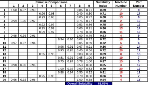
Fig. 4 shows a sample of these pair-wise comparisons, where the first 9 columns represent a comparison between each required part specification and machine capability for a given machine and part number. The machine number and part number are generated by the GA model and, hence, are the model chromosomes (last two columns).
Empty cells shown in the figure indicate that a machine is not capable of producing a given part specification. For example machine number 7 is a milling machine and can perform neither turning nor drilling operations (specifications 4 to 7 as indicated in Table 1).
The suitability index column indicates how suitable the machine is to produce the part’s required specifications. Furthermore, the overall suitability percentage is the average of all the pair-wise comparisons’ suitability index and should be maximized.
Suitability Machine Part
1 2 3 4 5 6 7 8 9 Index Number Number
1 1.00 0.97 0.93 0.85 0.71 0.89 7 8
2 0.96 0.98 0.40 0.50 0.71 10 17
3 0.93 0.98 0.05 0.77 0.68 13 6
4 0.99 1.00 0.97 0.75 0.77 0.90 2 10
5 0.92 0.97 0.53 0.56 0.75 10 12
6 0.95 0.99 0.60 0.91 0.86 13 14
7 0.99 0.97 0.78 0.68 0.86 11 13
8 0.98 0.95 0.91 1.00 0.79 0.93 4 9
9 0.94 0.96 0.08 0.92 0.72 18 6
10 0.97 0.97 0.94 0.05 0.69 0.72 5 6
11 0.96 0.91 0.67 0.91 0.86 17 14
12 0.93 0.95 0.45 0.56 0.72 20 17
13 0.95 0.93 0.83 0.83 0.89 8 18
14 0.81 0.91 0.65 1.00 0.84 19 7
15 0.75 0.97 0.78 1.00 0.87 15 5
16 0.98 0.90 0.96 0.53 0.88 0.85 3 12
17 1.00 0.92 0.60 0.63 0.79 20 12
18 0.88 0.94 0.50 0.92 0.81 18 11
19 0.95 0.98 0.70 0.80 0.86 9 7
20 0.96 0.92 0.96 1.00 0.88 0.94 4 15
[image:3.595.45.294.280.404.2]Overall Suitability 81.86% Pairwise Comparisons
Fig. 4: Sample of the pair-wise comparisons and their suitability indexes.
Finally, the model constraints and penalty factors section includes constraints used in the GA model as well as penalty to ensure that all model constraints are satisfied. These are discussed in further details later.
1) Model Mechanism
The GA model follows these steps to select the best machine(s) required to produce each part:
1) The GA model starts with generating a population of 100 machine and part chromosomes. Each machine chromosome contains 50 machines, and each part chromosome contains 50 parts.
2) The model compares each machine spec. with the corresponding part spec. and calculates the suitability index between the machine and part.
3) An overall suitability percentage is calculated (fitness function of the GA model).
4) Step 3 is repeated for all the first generation population. 5) The best 2% (1 – generation gap) of the population
chromosomes are copied directly to the next generation without crossover or mutation.
6) The rest of the population undergoes a crossover process in which a random number is generated. If the crossover rate is greater than or equal to the generated random number, then the crossover operator is applied.
7) Mutation is applied to the resulting offspring of the crossover process. A random number is generated. The mutation operator is applied only if the mutation rate (0.001) is greater or equal to the generated random number.
8) The offspring resulting form crossover and mutation processes plus the directly copied chromosomes from the previous generation, form the new generation. 9) The Gene Hunter program terminates the process if the
fitness function remains unchanged for 500 generations (stopping criteria). If not, it goes back to step 2.
2) Model Constraints and Penalty Factors
For the model to work properly, a set of constraints and penalty factors have to be applied. The model checks two values, which are the sum of the Yes/No column, and the sum of unsatisfied processes.
Yes/No column checks whether the part appeared in the comparisons or not and the unsatisfied processes checks whether each required process for a given part has a machine selected to perform it or not.
Thus there are two main constraints in that case these are: 1) The sum of the Yes/No column must be equal to the total
number of parts, which will prevent the model from ignoring parts (not including them in the comparisons). 2) The sum of unsatisfied processes must be equal to zero,
which will prevent the model from ignoring required manufacturing processes.
If any of these constraints were not satisfied, a penalty factor is applied which multiplies the overall suitability percentage by a large negative value; as shown in
[image:3.595.48.291.637.777.2]M T D M T D M T D
1 1 1 1 1 1 1 1 0 0 0
2 1 0 1 1 0 1 1 0 0 0
3 1 1 1 1 1 1 1 0 0 0
4 1 1 1 0 1 1 0 0 0 0
5 1 0 1 1 0 1 1 0 0 0
6 1 1 1 1 1 1 1 0 0 0
7 1 1 1 1 1 1 1 0 0 0
8 1 1 1 1 1 1 1 0 0 0
9 1 1 1 0 1 1 0 0 0 0
10 1 1 1 1 1 1 1 0 0 0
11 1 0 1 1 0 1 1 0 0 0
12 1 1 1 1 1 1 1 0 0 0
13 1 0 1 1 0 1 1 0 0 0
14 1 1 1 1 1 1 1 0 0 0
15 1 1 1 0 1 1 0 0 0 0
16 1 0 1 1 0 1 1 0 0 0
17 1 1 1 1 1 1 1 0 0 0
18 1 1 1 1 1 1 1 0 0 0
19 1 1 0 1 1 0 1 0 0 0
20 1 1 1 0 1 1 0 0 0 0
Total 20 15 19 16 15 19 16 0 0 0
processes numbe 50 Sum of Unsatisfied Constraints = 0
Penalty Factor = 1 Unsatisfied Processes Satisfied Processes
[image:4.595.46.292.47.227.2]Required Processes Part Yes/No
Fig. 5: Model constraints and penalty factors section for step 1 model.
B. Step 2: Forming Manufacturing Cells
Step two in the proposed procedure is to form manufacturing cells. The model purpose is to cluster the un-clustered part machine matrix obtained from the previous step. The model is divided into three sections. Section one is where the un-clustered data obtained from step one is located. Section two contains the distances calculations. Finally, section three is where the results of clustering are showed.
1) Model Mechanism
The model's main concept is to create a number of clustering centers and try to gather as much 1’s as possible around them by minimizing the total sum of distances between cluster centers and the 1’s.
The distance (d) between each cell value and the cluster center is calculated using the following formula:
2
2 ( )
)
(x X y Y
d = − + −
(1) Where:
x = the X-axis value of the cell.
y = the Y-axis value of the cell.
X = the X-axis value of the cluster center.
Y = the Y-axis value of the cluster center.
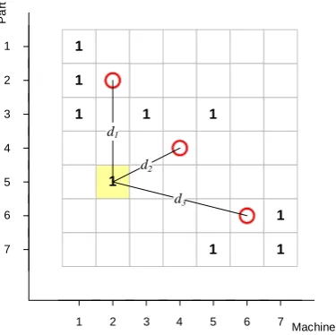
As there is more than one cluster center, the distance between the cell and each cluster center is calculated and the minimum distance is chosen, as indicated in
Fig. 6. Hence, distance equals:
) ,
min(d1 d2 dn
D= K (2)
Where:
D = minimum distance chosen.
n = number of clusters considered.
The model moves the locations of cluster centers, machines, and parts until minimum distance is obtained. To move any cell value, the entire values included in the row or column, in which that value belongs to, will be moved as well.
The chromosomes for the GA model are selected to be the machines and parts numbers, and the fitness function for the GA model is the minimization of the total sum of distances.
1
1
1
1 1
Pa
rt
Machine 1
1
1
1
1
d1
d2
d3
2 3 4 5 6 7
1
2
3
4
5
6
7
Fig. 6: Distance to cluster calculation.
The GA model follows these steps to solve the problem: 1) The GA model starts with generating a population of 200
machine and part chromosomes. Each machine chromosome contains 20 machines, and each part chromosome contains 20 parts.
2) The model calculates the distance between each cell value and all the cluster centers and choosing the least distance.
3) Calculate the total number of distances (fitness function).
4) Step two and three are repeated for all the first generation population.
5) The best 2% (1 – generation gap) of the population chromosomes are copied directly to the next generation without crossover or mutation.
6) The rest of the population undergoes a crossover process in which a random number is generated. If the crossover rate is greater than or equal to the generated random number, then the crossover operator is applied.
7) Mutation is applied to the resulting offspring of the crossover process. A random number is generated. The mutation operator is applied only if the mutation rate (0.001) is greater or equal to the generated random number.
8) The offspring resulting form crossover and mutation processes plus the directly copied chromosomes from the previous generation, form the new generation. 9) The Gene Hunter program terminates the process if the
fitness function remains unchanged for 500 generations (stopping criteria). If not, it goes back to step 2.
2) Model Constraints and Penalty factors
A number of constraints have to be applied for the model to work properly. The model checks if all the machines and parts appeared or not in the part-machine matrix. It also makes sure that every part and machine appears only once. This is achieved using two counters that are used to:
1) Show how many parts and machines that did not appear. 2) Show how many times each part and machine has
appeared.
[image:4.595.335.523.51.238.2]any part or machine appeared more than once in the matrix; the counters value is greater than zero and is multiplied by a large positive value.
The resulting value is then multiplied by the total distance value as a penalty. If all constraints have been satisfied (as in
Fig. 7) then the penalty value is equal to one.
Furthermore, the distance calculation formula given in equation (2) is modified to equation (3); thus, the distance from the cluster now increases exponentially. Hence, this acts a penalty to give more importance to lower distance values. The new distance formula is as follows:
) , min(d1d2 dn
e
D= K (3)
Machines
Parts15 11 19 7 9 8 16 1 13 5 17 10 3 20 18 14 2 4 12 6
5 1 1
13 1 1
19 1 1
7 1 1 1
8 1 1 1
16 1 1
1 1 1 1
18 1 1 1
4 1 1
14 1 1 1
6 1 1 1
17 1 1 1
3 1 1 1
12 1 1 1
2 1 1
10 1 1 1
11 1 1
9 1 1
20 1 1
15 1 1
1
# of Parts/Machines Not Selected # of Parts/Machines Selected than Once Total Number of Unsatisfied Constraints
Penalty for Unsatisfied Constraints
Fig. 7: Model constraints and penalty factors section for step 2 model.
V. COMPARING OTHER CLUSTERING TECHNIQUES TO THE
PROPOSED GENETIC ALGORITHM MODEL
To compare the GA model to other clustering techniques, five part-machine matrices from the literature are solved using the proposed model and the results are compared to other techniques.
Efficacy is used as a measure of performance [4, 9-17], where the closer the grouping efficacy is to 1, the better the grouping will be.
To calculate the grouping efficacy (µ) the following equation is used:
in out
N N
N N
0 1
1 1
+ − =
μ (4)
Where,
N1 = total number of 1's in the matrix.
N1out = total number of 1's outside the diagonal blocks
(cells).
N0in = total number of 0's inside the diagonal blocks (cells).
The proposed model has performed better than the other techniques found in literatures for part-machine matrices of size 7x11 and 14x24. Moreover, the results obtained from the proposed model for the remaining matrix sizes were the same as obtained from other techniques. These results are summarized in Table 2.
TABLE 2: DIFFERENT TECHNIQUES PERFORMANCE COMPARISONS.
No Sour
ce
Size ZODIAC GRAFICS MST GA TSP GA Proposed Approach
1
Kusiak &
Chow (
1987)
7x11 39.13 53.12 46.88 50 53.13
2
Boctor
(
1991)
7x11 70.37 70.37 70.37 70.37
3
Mo
iser &
T
aube (
1985)
10x10 70.59 70.59 70.59 70.59 70.59
4
Chan &
M
ilner
(
1982)
10x15 92 92 92 92 92
5
Askin &
Subr
am
anian
(1987
)
14x24 64.36 64.36 64.36 66.67
VI. CONCLUSION
A new two steps approach to solve the GT problem using GA is presented in this paper. Step one of the proposed GA approach is to identify the best machine(s) for each part based on machines and parts parameters (features). This step is ignored in most of the papers available in the literature, which only discuss the clustering problem without referring to the part-machine allocation problem, and the GT problem is solved assuming that the part-machine incidence matrix is already known.
Step two is to cluster the part-machine matrix obtained in step one to a selected number of clusters, and hence forming machine cells and part families. The proposed approach is very flexible to modify and has the advantage of allowing the user to select and test different numbers of manufacturing cells, which is very useful in many cases.
[image:5.595.50.550.65.427.2]REFERENCES
[1] M. P. Groover, Automation, Production Systems, and Computer
Integrated Manufacturing: Prentice-Hall International, Inc., 1987. [2] D. D. Bedworth, Hendersen,M. P., and Wolfe, P. M., Computer
Integrated Design and Manufacturing: McGraw-Hill, Inc., 1991. [3] J. R. King, "Machine-component group formation in group
technology," Omega, vol. 8, pp. 193-199, 1980.
[4] H. M. Chan, and Milner, D. A., "Direct clustering algorithm for group formation in cellular manufacturing," Journal of Manufacturing Systems, vol. 1, pp. 65-75, 1982.
[5] F. Glover, "Tabu Search — Part I," ORSA Journal on Computing, vol. 1, pp. 190-206, 1989.
[6] F. Glover, "Tabu Search — Part II," ORSA Journal on Computing, vol. 2, pp. 4-32, 1990.
[7] R. P. Lippman, "An introduction to computing with neural nets.,"
IEEE ASSP magazine, pp. 4-22, 1987.
[8] V. Cerny, "A thermodynamical approach to the travelling salesman problem: an efficient simulation algorithm," Journal of Optimization Theory and Applications, vol. 45, pp. 41-51, 1985.
[9] G. Srinivasan, "A clustering algorithm for machine cell formation in group technology using minimum spanning trees," International Journal of Production Research, vol. 32, pp. 2149-2158, 1994. [10] G. C. Onwubolu, and Mutingi, M., "A genetic algorithm approach to
cellular manufacturing systems," Computers and Industrial Engineering, vol. 39, pp. 125-144, 2001.
[11] A. Kusiak, Chow, W. , "Efficient solving of the group technology problem," Journal of Manufacturing Systems, vol. 6, pp. 117-124, 1987.
[12] F. Boctor, "A linear formulation of the machine-part cell formation problem," International Journal of Production Research, vol. 29, pp. 343-356, 1991.
[13] C. T. Moiser, and Taube, L., "The facets of group technology and their impact on implementation," OMEGA, vol. 13, pp. 381-391, 1985. [14] R. G. Askin, and Subramanian, S. , "A cost based heuristic for group
technology configuration," International Journal of Production Research, vol. 25, pp. 101-113, 1987.
[15] M. Chandrasekharan, P., Rajagopalan, R., "ZODIAC - An algorithm for concurrent formation of part families and machine cells.,"
International journal of Production Research, vol. 25, pp. 835-850, 1987.
[16] G. Srinivasan, Narendran, T. T., "GRAFICS - A nonhierarachical clustering algorithm for group technology " International journal of Production Research., vol. 29, pp. 463-478, 1991.
[17] C. H. Cheng, Gupta, Y. P., Lee, W. H., and Wong, K. F., "A TSP-based heuristic for forming machine groups and part families. ,"