Exceptionality and Natural Language Learning

Exceptionality and Natural Language Learning

Mihai Rotaru

Diane J. Litman

Computer Science Department

University of Pittsburgh

Pittsburgh, PA 15260

mrotaru, litman @cs.pitt.edu

Abstract

Previous work has argued that memory-based learning is better than abstraction-based learn-ing for a set of language learnlearn-ing tasks. In this paper, we first attempt to generalize these re-sults to a new set of language learning tasks from the area of spoken dialog systems and to a different abstraction-based learner. We then examine the utility of various exceptionality measures for predicting where one learner is better than the other. Our results show that generalization of previous results to our tasks is not so obvious and some of the exceptional-ity measures may be used to characterize the performance of our learners.

1 Introduction

2

Our paper is a follow-up of the study done by

Daele-mans et al. (1999) in which the authors show that keep-ing exceptional trainkeep-ing instances is useful for increasing generalization accuracy when natural lan-guage learning tasks are involved. The tasks used in their experiments are: grapheme-phoneme conversion, part of speech tagging, prepositional phrase attachment and base noun phrase chunking. Their study provides empirical evidence that editing exceptional instances leads to a decrease in memory-based learner perform-ance. Next, the memory-based learner is compared on the same tasks with a decision-tree learner and their results favor the memory-based learner. Moreover, the authors provide evidence that the performance of their memory-based learner is linked to its property of hold-ing all instances (includhold-ing exceptional ones) and gen-eral properties of language learning tasks (difficultness in discriminating between noise and valid exceptions and sub-regularities for those tasks).

We continue on the same track by investigating if their results hold on a different set of tasks. Our tasks

come from the area of spoken dialog systems and have smaller datasets and more features (with many of the features being numeric, in contrast with the previous study that had none). We observe in our experiments with these tasks a much smaller exceptionality measure range compared with the previous study. Our results indicate that the previous results do not generalize to all our tasks.

An additional goal of our research is to investigate a new topic by looking into whether exceptionality meas-ures can be used to characterize the performance of our learners: a memory-based learner (IB1-IG) and a rule-based learner (Ripper). Our results indicate that for some of the exceptionality measures we will examine, IB1-IG is better for predicting typical instances while Ripper is better for predicting exceptional instances.

We will use the following conventions throughout the paper. The term “exceptional” will be used to label instances that do not follow the rules that characterize the class they are part of (in language learning terms, they are “bad” examples of their class rules). We will use “typical” as the antonym of this term; it will label instances that are good examples of their class rules. The fact that an instance is typical should not be con-fused with an exceptionality measure we will use that has the same name (typicality measure).

Learning

methods

We will use in our study the same memory-based learner that was used in the previous study: IB1-IG. The abstraction-based learner used in the previous study was C5.0 (a commercial implementation of the C4.5 deci-sion tree learner). In our study we will use a rule-based learner, Ripper. Although the two abstraction-based learners are different, they share many features (many techniques used in rule-based learning have been adapted from decision tree learning (Cohen, 1995))1_.

2.1

IB1-IG

Our memory-based learner is called IB1-IG and is part of TiMBL, a software package developed by the ILK Research Group, Tilburg University and the CNTS Re-search Group, University of Antwerp. TiMBL is a col-lection of memory-based learners that sit on top of the classic k-NN classification kernel with added metrics, algorithms, and extra functions.

Memory-based reasoning is based on the hypothesis that humans, in order to react to a new situation, first compare the new situation with previously encountered situations (which reside in their memory), pick one or more similar situations, and react to the new one based on how they reacted to those similar situations. This type of learning is also called lazy learning because the learner does not build a model from the training data. Instead, typically, the whole training set is stored. To predict the class for a new instance, the lazy learner compares it with stored instances using a similarity met-ric and the new instance class is determined based on the classes of the most similar training instances. At the algorithm level, lazy learning algorithms are versions of k-nearest neighbor (k-NN) classifiers.

IB1-IG is a k-NN classifier that uses a weighted overlap metric, where a feature weight is automatically computed as the Information Gain (IG) of that feature. The weighted overlap metric for two instances X and Y

is defined as:

∑

=

=

∆ n

i

i i

i x y

w Y

X

1

) , ( )

,

( δ (1)

where:

i i

i i i i

i i

i i

y x

y x min max

y x abs

y x

≠ = 

     

− −

=

if if

else numeric, if

1 0

) (

) , (

δ

Information gain is computed for every feature in isolation by computing the difference in uncertainty between situations with or without knowledge of the feature value (for more information, see Daelemans et al., 2001). These values describe the importance of that feature in predicting the class of an instance and are used as feature weights.

2.2

3

3.1

Ripper

Ripper is a fast and effective rule-based learner devel-oped by William Cohen (Cohen, 1995). The algorithm has an overfit-and-simplify learning strategy: first an initial rule set is devised by overfitting a part of the training set (called the growing set) and then this rule set is repeatedly simplified by applying pruning opera-tors and testing the error reduction on another part of the

training set (called the pruning set). Ripper produces a model consisting of an ordered set of if-then rules.

There are several advantages to using rule-based learners. The most important one is the fact that people can understand relatively easy the model learned by a rule-based learner compared with the one learned by a decision-tree learner, neural network or memory-based learner. Also, domain knowledge can be incorporated in a rule-based learner by altering the type of rules it can learn. Finally, rule-based learners are relatively good at filtering the potential noise from the training set. But in the context of natural language learning tasks where distinguishing between noise and exceptions and sub-regularities is very hard, this filtering may result in a decrease in accuracy. In contrast, memory-based learn-ers, by keeping all instances around (including excep-tional ones), may have higher classification accuracy for such tasks.

Exceptionality

measures

One of the main disadvantages of memory-based learn-ing is the fact that the entire trainlearn-ing set is kept. This leads to serious time and memory performance draw-backs if the training set is big enough. Moreover, to improve accuracy, one may want to have noisy in-stances present in the training set pruned. To address these problems there has been a lot of work on trying to edit part of the training set without hampering the accu-racy of the predictor. Two types of editing can be done. One can edit redundant regular instances (because the training set contains a lot of similar instances for that class) and/or unproductive instances (the ones that pre-sent irregularities with respect to the training set space). There are many measures that capture both types of instances. We will use the ones from the previous study (typicality and class prediction strength) and a new one called local typicality. Even though these measures were devised with the purpose of editing part of the training set, they are used in our study and the previous study to point out instances that should not be removed, at least for language learning tasks.

Typicality

weighted Manhattan distance from (1). Thus, our simi-larity measure will be defined as:

∑

=

− = n

i i i i

y x w

Y X sim

1

)) , ( 1 ( )

,

( δ

For every instance X, a subset of the dataset called

family of X, Fam(X), is defined as being all instances from the dataset that have the same class as X. All re-maining instances form the unrelated instances subset,

Unr(X). Then, intra-concept similarity is defined as the

average similarity between X and instances from

Fam(X) and inter-concept similarity as the average similarity between X and instances from Unr(X).

∑

=

= | ( |)

1

) ) ( , ( |

) ( |

1 )

( Fam X

i

i

X Fam X sim X

Fam X

Intra

∑

=

= | ( |)

1

) ) ( , ( |

) ( |

1 )

( Unr X

i

i

X Unr X sim X

Unr X

Inter

Finally, typicality of an instance X is defined as the ratio of its intra-concept and inter-concept similarity.

) (

) ( )

(

X Inter

X Intra X

Typicality =

The typicality values are interpreted as follows: if the value is higher than 1, then that instance has an in-tra-concept similarity higher than inter-concept similar-ity, thus one can say that the instance is a good example of its class (it is a typical instance). A value less than 1 implies the opposite: the instance is not a good example of its class (it is an exceptional instance). Values around 1 are called by Zhang boundary instances since they seem to reside at the border between concepts.

3.2

3.3

Class prediction strength

Another measure used in the previous study is the class prediction strength (CPS). This measure tries to capture the ability of an instance to predict correctly the class of a new instance. We will employ the same CPS defini-tion used in the previous study (the one proposed by Salzberg (1990)). In the context of k-NN, predicting the class means, typically, that the instance is the closest neighbor for a new instance. Thus the CPS function is defined as the ratio of the number of times our instance is the closest neighbor for an instance of the same class and the number of times our instance is the closest neighbor for another instance regardless of its class. A CPS value of 1 means that if our instance is to influence another instance class (by being its closest neighbor) its influence is good (in the sense that predicting the class using our instance class will result in an accurate predic-tion). Thus our instance is a good predictor for our class, i.e. it is a typical instance. In contrast, a value of 0 indi-cates a bad predictor for the class and thus labels an exception instance. A value of 0.5 will correspond to instances at the border between concepts.

Unlike typicality, when computing CPS, we can en-counter situations when its value is undefined (zero di-vided by zero). This means that the instance is not the closest neighbor for any other instance. Since there is no clear interpretation of instance properties in this case, we will set its CPS value to a constant higher than 1 (no particular meaning of the value, just to recognize it in our graphs).

Local typicality

While CPS captures information very close to an in-stance, typicality as defined by Zhang captures informa-tion from the entire dataset. But this may not be the most desirable measure in cases such as those when a concept is made of at least two disjunctive clusters. Consider the example from Figure 1. For an instance in the center of cluster A1, its similarity with instances

from the same cluster is very high but very low with instances from cluster A2. At the same time, its

similar-ity with instances from class B is somewhere between above two values. When everything is averaged, in-stance intra-concept and inter-concept similarity have comparable values thus leading to a typicality value around 1 even if the instance is highly typical for the cluster A1.

A1

To address this problem, we changed the definition of Fam(X) and Unr(X). Instead of considering all in-stances from the dataset when building the two subsets, we will be using only instances from a vicinity of our instance. The typicality computed using these new sub-sets will be called local typicality. To define the vicin-ity, we used again the similarity metric. When two instances are identical, their similarity has the maximum value which is the sum of all feature weights. An in-stance is in the vicinity of another inin-stance if and only if their similarity has a value higher than a given percent of maximum similarity value (using this definition of vicinity instead of a specified number of nearest neighbors, makes our exceptionality measure adaptive to the density of the local neighborhood). For our data-sets, a percent value of 90% yields the best results fur-nishing a measure that is different from both typicality and CPS.

Like CPS, division by zero can appear when com-puting local typicality. This means that inter-concept

B

A2

similarity is zero and this can only happen if there is no instance with a different class in the vicinity of our in-stance. In this case, if the intra-concept similarity is higher than 0 (there is at least one instance from the same class in the vicinity) we set the local typicality to a maximum value, while if the intra-concept similarity is 0, then we set the typicality to a minimum value (no one in the vicinity of this instance is a good indication of an exceptional instance). When inter-concept similarity is higher than 0, we will set the local typicality to a mini-mum value if its intra-concept similarity is 0 (so that we will not have a big gap between local typicality values). Minimum and maximum values are computed as values to the left and right of the local typicality interval for non-exceptional cases.

We can rank our exceptionality measures by the level of information they capture (from most general to most local): typicality, local typicality and CPS.

4 Language learning tasks

The tasks we will be using in our study come from the area of spoken dialog systems (SDS). They were all designed as methods for potentially improving the dia-log manager of a SDS system called TOOT (Litman and Pan, 2002). This system provides access to train infor-mation from the web via telephone and it was developed for the purpose of comparing differences in dialog strat-egy.

Our tasks are: (1) Identifying user corrections (ISCORR), (2) Identifying correction-aware sites (STATUS), (3) Identifying concept-level speech recog-nition errors (CABIN) and (4) Identifying word-level speech recognition errors (WERBIN). The first task is a binary classification task that labels each user turn as to whether or not it is an attempt from the user to correct a prior system recognition failure. The second task is a 4-way classification task that extends the previous one with whether or not the user is aware the system made a recognition error. The four classes are: normal user turn, user only tries to correct the system, user is only aware of a system recognition error, and user is both aware of and tries to correct the system error. The third and the fourth tasks are binary classification tasks that try to predict the system speech recognition accuracy when recognizing a user turn. CABIN measures a binary ver-sion of the Concept Accuracy (percent of semantic con-cepts recognized correctly) while WERBIN measures a binary version of the Word Error Rate (percent of words recognized incorrectly).

Data for our tasks was gathered from a corpus of 2,328 user turns from 152 dialogues between human subjects and TOOT. The features used to represent each user turn include prosodic information, information from the automatic speech recognizer, system condi-tions and dialog history. Then, each user turn was

la-beled with respect to every classification task. Even though our classification tasks share the same data, there are clear differences between them. ISCORR and STATUS both deal with user corrections which is quite different from predicting speech recognition errors (handled in WERBIN and CABIN). Moreover, one will expect very little noise or no noise at all when manually annotating WERBIN and CABIN. For more information on our tasks and features, see (Litman et al., 2000; Hirschberg et al., 2001; Litman et al., 2001).

There are a number of dimensions where our tasks differ from the tasks from the previous study. First of all our datasets are smaller (2,328 instances compared with at least 23,898). Second, the number of features used is much bigger than the previous study (141 compared with 4-11). Moreover, many features from our datasets are numeric while the previous study had none. These differences will also reflect on our exceptionality meas-ures values. For example, the smallest range for typical-ity in the previous study was between 0.43 and 10.57 while for our tasks it is between 0.9 and 1.1. To explore these differences we varied the feature set used. Instead of using all the available features (this feature set is called All), we restricted the feature set by using only non-numeric features (Nonnum – 22 features). The typi-cality range increased when using this feature set (0.77-1.45), but the number of features used was still larger than the previous study. For this reason, we next de-vised two set of features with only 9 (First9) and 15 features (First15). The features were selected based on their information gain (see section 2.1).

Before proceeding with our results, there is one more thing we want to mention. At least half of our in-stances have one or more missing values and while the Ripper implementation offered a way to handle them, there was no default handling of missing values in the IB1-IG implementation. Thus, we decided to replace missing values ourselves before presenting the datasets to our learners. In particular there are two types of miss-ing values: genuine missmiss-ing values (no value was pro-vided; we will refer to them as missing values) and undefined values. Undefined values come from features that are not defined in that user turn (for example, in the first user turn, most of the dialog history features were undefined because there was no previous user turn).

the values provided comparable results. For our experi-ments, missing values were replaced with a value to the right of the interval for that feature and undefined val-ues were replaced with a value to the left of that inter-val.

5 Results

5.1

In 5.1 we reproduce the editing and comparison experi-ments from the previous study to see if their results gen-eralize to our tasks. In 5.2, we move to our next goal: characterizing learners’ performance using exceptional-ity measures. Both learners were run using default pa-rameters2_.

Natural language learning and memory-based learning

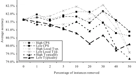
First, we performed the editing experiments from the previous study. The purpose of those experiments was to see the impact of editing exceptional and typical in-stances on the accuracy of the memory-based learner. Since our datasets were small, unlike the previous study which performed editing only on the first train-test par-tition of a 10-fold cross validation, we performed the editing experiment on all partitions of a 10-fold cross validation. For every fold, we edited 0, 1, 2, 5, 10, 20, 30, 40 and 50% of the training set based on extreme values of all our exceptionality criteria. Accuracy after editing a given percent was averaged among all folds (there is a significant difference in accuracies among folds but all folds exhibit a similar trend with the aver-age). Figure 2 shows our results for the ISCORR dataset

79.0% 79.5% 80.0% 80.5% 81.0% 81.5% 82.0% 82.5% 83.0%

0 1 2 5 10 20 30 40 50

Percentage of instances removed

A

ver

ag

e a

cc

ur

acy

High CPS Low CPS High Local T yp. Low Local T yp. High T ypicality Low T ypicality

Figure 2. IB1-IG average accuracy after editing a given percent of the training set based on high and low extremes of all exceptionality

measures (ISCORR dataset with all features)

2 _{We performed parameter tuning experiments for both} predic-tors: for every fold of a 10-fold cross validation, part of the training set was used as a validation set (for tuning parame-ters). Our results indicate that the tuned parameters depend on the fold used and there was no clear gain to accuracy from tuning (in some cases there was even loss in accuracy). Inte-grating tuned parameters with our leave-one-out experiments presents additional problems.

using six types of editing (editing based on low and high value for all three criteria). In contrast with the previous study, where for all tasks even the smallest editing led to significant accuracy decreases, for our task there was no clear decrease in performance. Moreover, for some criteria (like low local-typicality) we can even see an initial increase in performance. Only after editing half of the training set is there a clear decrease in perform-ance for all editing criteria on this task.

Editing experiments for the other dataset-feature set combinations yield similar results.

Next, we compared the memory-based learner with our abstraction-based learner on all tasks. Since the datasets were relatively small, we performed leave-one-out cross validations. Table 1 summarizes our results. The baseline used is the majority class baseline. First, we run the predictors on all tasks using all features. In contrast with the previous study which favored the memory-based learner for almost all their tasks, our results favor IB1-IG for only two of the four tasks (ISCORR and STATUS). In Section 4, we mentioned that the typicality range for our tasks was very small compared with the previous study. Contrary to what we

expected, the tasks where IB1-IG performed better were the ones with smaller typicality range. To investigate the typicality range impact on our predictors, we tried to make our datasets similar to the datasets from the previ-ous study by tackling the feature set. We eliminated all numeric features (since the tasks from the previous study had none) and performed experiments on the tasks that had the less typicality range (again, ISCORR and STATUS). Again, when typicality range was increased, even though there were no numeric features, IB1-IG performed worse than Ripper. IB1-IG error rate in-creased when using only non-numeric features for both tasks compared with the error rate when using all fea-tures. This observation led us to assume that, at least for IB1-IG, some of the relevant features for classification were numeric and they were not present in our feature set. Thus, we selected two sets of features (First9 and

First15) based on the features’ relevance and performed the experiments again on the ISCORR dataset. We can

Error rate

Data-Feat. set IB1-IG Ripper Baseline

Typicality range

[image:5.612.79.296.457.579.2]

Iscorr-All 14.99% 16.15% 28.99% 0.94 - 1.06 Status-All 22.25% 23.71% 43.04% 0.96 - 1.10 Cabin-All 13.10% 12.11% 30.50% 0.90 - 1.12 Werbin-All 17.65% 11.90% 39.22% 0.90 - 1.10 Iscorr-Nonnum 17.01% 16.24% 28.99% 0.81 - 1.49 Status-Nonnum 23.93% 21.99% 43.04% 0.88 - 1.62 Iscorr-First9 17.78% 16.07% 28.99% 0.86 - 1.17 Iscorr-First15 14.69% 14.95% 28.99% 0.88 - 1.14

observe that as the number of relevant features is in-creased, the error rate for both predictors and the typi-cality range are decreasing and IB1-IG takes the lead when the First15 feature set is used. Our results indicate that the predictor that performs better depends on the task, the number of features and the type of features we use.

To explore why the previous study’s results do not generalize in our case, we are planning to replicate these experiments on the dialog-act tagging task on the Switchboard corpus (a task more similar in size and feature types with the previous study than our tasks but still in the area of spoken dialog systems – see Shriberg et al. (1998)).

5.2

Characterizing learners’ performance using exceptionality measures

The next goal of our study was to see if we can charac-terize the performance of our predictors on various classes of instances defined by our exceptionality crite-ria. In other words, we wanted to try to answer ques-tions like: is IB1-IG better at predicting exceptional instances than Ripper? How about typical instances? Can we combine the two learners and select between them based on the instance exceptionality?

To answer these questions, we performed the leave-one-out experiments described above and recorded for every instance whether our predictors predicted it cor-rectly or incorcor-rectly. Next, we computed the exception-ality of every instance using all three measures. Figure 3 shows the exceptionality distribution using the typicality measure for the ISCORR dataset with all features3_{. The}

0 50 100 150 200 250 300 350 400 450

0.94 0.95 0.96 0.97 0.98 0.99 1.00 1.01 1.02 1.03 1.04 1.05 1.06 T ypicality

Fr

eque

nc

y

[image:6.612.320.538.215.338.2]

IB1-IG Ripper Full dataset

Figure 3. Typicality distribution for all instances, instances correctly predicted by IB1-IG and instances correctly predicted by Ripper

(ISCORR dataset with all features)

typicality distributions of all instances from the ISCORR dataset, of instances correctly predicted by IB1-IG, and of instances correctly predicted by Ripper are plotted in the figure. The graph shows that for this dataset there are a lot of boundary instances, very few exceptional instances and few typical instances. The

typicality range for all our datasets (usually between 0.85 and 1.15) is far less than the one from the previous study (0.43 up to 10 or even 3500). According to Zhang (1992) hard concepts are often characterized by small typicality spread. Moreover, small typicality spread is associated with low accuracy in predicting.

3 _{For other dataset-feature set combination graphs see:} http://www.cs.pitt.edu/~mrotaru/exceptionality

Figure 4 shows the same information as Figure 3, but instead of plotting the count, we plot the percentage of the instances with typicality between a given interval that have been correctly classified by one of the predic-tors. We can observe that accuracy of both predictors increases with typicality. That is, the more typical the

0% 10% 20% 30% 40% 50% 60% 70% 80% 90% 100%

0.94 0.95 0.96 0.97 0.98 0.99 1.00 1.01 1.02 1.03 1.04 1.05 1.06 Typicality

C

or

re

ctly

p

re

dic

te

d

p

er

ce

nta

ge

IB1-IG Ripper

Figure 4. Percent of instances predicted correctly by IB1-IG and Rip-per based on instance typicality (ISCORR dataset with all features)

instance, the more reliable the prediction; the more ex-ceptional the instance, the more unreliable the predic-tion. This observation holds for all our dataset-feature set combinations. It is not clear for the ISCORR dataset whether one predictor is better than the other based on the typicality. But for datasets CABIN and WERBIN where, overall, IB1-IG did worse than Ripper, the same graph (see Figure 5) shows that IB1-IG’s accuracy is worse than Ripper’s accuracy when predicting low typi-cality instances4_{. Given the problems with typicality if}

the concepts we want to learn are clustered, we decided

0% 10% 20% 30% 40% 50% 60% 70% 80% 90% 100%

0.89 0.91 0.93 0.94 0.96 0.98 1.00 1.02 1.04 1.06 1.07 1.09 1.11 T ypicality

C

orr

ec

tly

p

re

di

ct

ed

-

pe

rc

en

ta

ge

[image:6.612.78.296.452.582.2]

IB1-IG Ripper

Figure 5. Percent of instances predicted correctly by IB1-IG and Rip-per based on instance typicality (CABIN dataset with all features)

[image:6.612.319.536.503.629.2]

to investigate if this observation holds for other excep-tionality measures.

We continued the experiments on the other excep-tionality measures hoping to get more insight into the trend observed for typicality. Indeed, Figure 6 (same as Figure 4 but using the CPS instead of typicality) shows the same trend: IB1-IG is worse than Ripper when dicting exceptional instances and it is better when pre-dicting typical instances. The accuracy curves of the two predictors seem to cross at a CPS value of 0.5, which corresponds to boundary instances. Undefined CPS values (0/0) are assigned a value above 1 (the rightmost point on the graph). Ripper was the one that offered higher accuracy in predicting instances with undefined CPS value for almost all datasets (although not in Figure 6). The result holds for all our dataset-feature set combinations.

0% 10% 20% 30% 40% 50% 60% 70% 80% 90% 100%

0.00 0.08 0.17 0.25 0.34 0.42 0.51 0.59 0.68 0.76 0.85 0.93 1.02 CPS

Pr

ed

ic

te

d

co

rr

ect

ly

p

er

cen

ta

ge

[image:7.612.79.296.269.397.2]

IB1-IG Ripper

Figure 6. Percent of instances predicted correctly by IB1-IG and Rip-per based on instance CPS (ISCORR dataset with all features)5

The experiments with local typicality yield the same results: Ripper constantly outperforms IB1-IG for ex-ceptional instances and they switch places for typical instances (see Figure 7). Again, the accuracy curves cross at boundary instances (local typicality value of 1) and the same observation holds for all dataset-feature set combinations.

0% 10% 20% 30% 40% 50% 60% 70% 80% 90% 100%

0.91 0.92 0.93 0.95 0.96 0.97 0.99 1.00 1.01 1.03 1.04 1.05 1.07 Local T ypicality

C

or

rect

ly

p

red

ic

te

d

p

er

cen

ta

ge

[image:7.612.319.527.399.563.2]

IB1-IG Ripper

Figure 7. Percent of instances predicted correctly by IB1-IG and Ripper based on instance local typicality

(ISCORR dataset with all features)

5 _{Abrupt movements in curves are caused by small number of} instances in that class. We expect that a larger dataset will smooth our graphs.

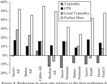
We computed what could be the reduction in error rate if we were to employ both predictors and decide between them based on the instance exceptionality measure. In other words, Ripper prediction was used for exceptional instances and for the left-hand side bound-ary instances (CPS less than 0.5; typicality less than 1; local typicality less than 1); otherwise IB1-IG prediction was used. The lower bound of this reduction is when we perfectly know which of the predictors offer the correct prediction (in other words the error rate is the number of times both learners furnished wrong predictions). Figure 8 plots the reduction in error rate achieved when decid-ing between predictors based on typicality, CPS, local typicality and perfect discrimination. The reduction is relative to the best performer on that task. While dis-criminating based on typicality offered no improvement relative to the best performer, CPS was able to con-stantly achieve improvement and local typicality im-proved in six out of eight cases. CPS imim-proved the error rate of the best performer by decreasing it by 1.33% to 3.18% (absolute percentage). In contrast with CPS, local typicality offered, for the cases when it improved the accuracy, more improvement decreasing the error rate by up to 4.94% (absolute percentage). A possible expla-nation of this difference can be the fact that local typi-cality captures much more information than CPS (vicinity-level information compared with information very close to the instance).

-20% -10% 0% 10% 20% 30% 40% 50% 60%

Is

co

rr-Al

l

Sta

tu

s-Al

l

Ca

bi

n-A

ll

We

rb

in

-Al

l

Is

co

rr-N

onnum _Statu

s-N

onnum Isco

rr-Fir

st9

Is

co

rr-Fir

st1

5

T ypicality CPS

Local Typicality Perfect Discr.

Figure 8. Reduction in error rate relative to the best performer for typicality, CPS, local typicality and prefect discrimination

[image:7.612.77.295.509.641.2]

5.3

Current directions

The previous section showed that we can improve the overall accuracy on our datasets if we combine the pre-diction generated by our learners based on the excep-tionality measure of the new instance. Unfortunately, all our exceptionality measures require the class of the in-stance. Moreover, for binary classification tasks, since all exceptionality criteria are a ratio, changing the in-stance class will turn an exceptional inin-stance into a typical instance.

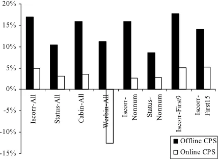
To move our results from offline to online, we con-sidered interpolating the exceptionality value for an instance based on its neighbors’ exceptionality values (the neighbors from the training set). We performed a very simple interpolation by using the exceptionality value of the closest neighbor (relative to equation (1)). While previous observations are not obvious anymore in online graphs (there is no clear crossing at boundary instances), there is a small improvement over the best predictor. Figure 9 shows that even for this simple in-terpolation there is a small reduction in almost all cases in error rate relative to the best performer when using online CPS (interpolated CPS).

-15% -10% -5% 0% 5% 10% 15% 20%

Is

co

rr

-A

ll

Sta

tu

s-A

ll

C

abi

n-A

ll

W

erbi

n-A

ll

Is

co

rr

-N

onnum _Statu

s-N

onnum

Is

co

rr

-F

ir

st

9

Is

co

rr-Fi

rs

t1

5

[image:8.612.77.291.350.506.2]

Offline CPS Online CPS

Figure 9. Reduction in error rate relative to the best performer for offline CPS and online CPS

We are currently investigating more complicated in-terpolation strategies like learning of a model from the training set that will predict the exceptionality value of an instance based on its closest neighbors.

6 Conclusions

In this paper we attempted to generalize the results of a previous study to a new set of language learning tasks from the area of spoken dialog systems. Our experi-ments indicate that previous results do not generalize so obviously to the new tasks. Next, we showed that some exceptionality measures can be used as means to im-prove the prediction accuracy on our tasks by combin-ing the prediction of our learners based on measures of instance exceptionality. We observed that our

memory-based learner performs better than the rule-memory-based learner on typical instances and they exchange places for excep-tional instances. We also showed that there is potential for moving these results from offline to online by per-forming a simple interpolation. Future work needs to address more complicated methods of interpolation, comparison between our method and other attempts to combine rule-based learning and memory-based learn-ing (Domlearn-ingos, 1996; Goldlearn-ing and Rosenbloom, 1991), comparison with ensemble methods, and whether the results from this paper generalize to other spoken dialog corpora.

Acknowledgements

We would like to thank Walter Daelemans and Antal van den Bosch for starting us on this work.

References

William Cohen. 1995. Fast effective rule induction. ICML. Walter Daelemans, Antal van den Bosch, and Jakub Zavrel.

1999. Forgetting exceptions is harmful in language learning. Machine Learning 1999, 34 :11-43.

Walter Daelemans, Jakub Zavrel, Ko van der Sloot, and Antal van den Bosch. 2001. TiMBL: Tilburg Memory Based Learner, version 4.1, Reference Guide. ILK Technical Report – ILK 01-04.

Pedro Domingos. 1996. Unifying Instance-Based and Rule-Based Induction. Machine Learning 1996, 24:141-168 Andrew R. Golding and Paul S. Rosenbloom. 1991. Improving

Rule-Based Systems Through Case-Based Reasoning. Proc. AAAI.

Julia Hirschberg, Diane J. Litman, and Marc Swerts. 2001.

Identifying User Corrections Automatically in Spoken Dialogue Systems. Proc. NAACL.

Diane J. Litman, Julia Hirschberg, and Marc Swerts. 2000.

Predicting Automatic Speech Recognition Performance Using Prosodic Cues. Proc. NAACL.

Diane J. Litman, Julia Hirschberg, and Marc Swerts. 2001.

Predicting User Reactions to System Error. Proc. ACL. Diane J. Litman, Shimei Pan. 2002. Designing and Evaluating

an Adaptive Spoken Dialogue System. User Modeling and User-Adapted Interaction, 12(2/3):111-137.

Salzberg, S. 1990. Learning with nested generalised exemplars. Kluwer Academic Publishers.

Elizabeth Shriberg, Rebecca Bates, Paul Taylor, Andreas Stolcke, Klaus Ries, Daniel Jurafsky, Noah Coccaro, Rachel Martin, Marie Meteer, and Carol Van Ess-Dykema. 1998. Can prosody aid the automatic classification of dialog acts in conversational speech?. Language and Speech 41:439—487.