Greedy Decoding for Statistical Machine Translation in Almost Linear Time

Greedy Decoding for Statistical Machine Translation in Almost Linear Time

Ulrich Germann

USC Information Sciences Institute

Marina del Rey, CA

germann@isi.edu

Abstract

We present improvements to a greedy decod-ing algorithm for statistical machine translation that reduce its time complexity from at least cubic (

when applied na¨ıvely) to

prac-tically linear time1 _{without sacrificing}

trans-lation quality. We achieve this by

integrat-ing hypothesis evaluation into hypothesis cre-ation, tiling improvements over the translation hypothesis at the end of each search iteration, and by imposing restrictions on the amount of word reordering during decoding.

1

Introduction

Most of the current work in statistical machine translation builds on word replacement models developed at IBM in the early 1990s (Brown et al., 1990, 1993; Berger et al., 1994, 1996). Based on the conventions established in Brown et al. (1993), these models are commonly referred to as the (IBM) Models 1-5.

One of the big challenges in building actual MT sys-tems within this framework is that of decoding: finding

the translation candidate that maximizes the translation

probability

for the given input . Knight (1999)

has shown the problem to be NP-complete.

Due to the complexity of the task, practical MT sys-tems usually do not employ optimal decoders (that is, decoders that are guaranteed to find an optimal solution within the constraints of the framework), but rely on ap-proximative algorithms instead. Empirical evidence sug-gests that such algorithms can perform resonably well. For example, Berger et al. (1994), attribute only 5% of the translation errors of their Candide system, which uses

1

Technically, the complexity is still. However, the

quadratic component has such a small coefficient that it does not have any noticable effect on the translation speed for all reasonable inputs.

a restricted stack search, to search errors. Using the same evaluation metric (but different evaluation data), Wang and Waibel (1997) report search error rates of 7.9% and 9.3%, respectively, for their decoders.

Och et al. (2001) and Germann et al. (2001) both im-plemented optimal decoders and benchmarked approxi-mative algorithms against them. Och et al. report word error rates of 68.68% for optimal search (based on a vari-ant of the A* algorithm), and 69.65% for the most re-stricted version of a decoder that combines dynamic pro-gramming with a beam search (Tillmann and Ney, 2000). Germann et al. (2001) compare translations obtained by a multi-stack decoder and a greedy hill-climbing al-gorithm against those produced by an optimal integer programming decoder that treats decoding as a variant of the traveling-salesman problem (cf. Knight, 1999). Their overall performance metric is the sentence error rate (SER). For decoding with IBM Model 3, they report SERs of about 57% (6-word sentences) and 76% (8-word sentences) for optimal decoding, 58% and 75% for stack decoding, and 60% and 75% for greedy decoding, which is the focus of this paper.

All these numbers suggest that approximative algo-rithms are a feasible choice for practical applications.

The purpose of this paper is to describe speed improve-ments to the greedy decoder mentioned above. While ac-ceptably fast for the kind of evaluation used in Germann

et al. (2001), namely sentences of up to 20 words, its

speed becomes an issue for more realistic applications. Brute force translation of the 100 short news articles in Chinese from the TIDES MT evaluation in June 2002 (878 segments; ca. 25k tokens) requires, without any of the improvements described in this paper, over 440

CPU hours, using the simpler, “faster” algorithm

(de-scribed below). We will show that this time can be re-duced to ca. 40 minutes without sacrificing translation quality.

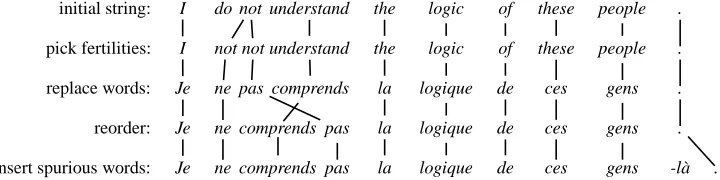
initial string: I do not understand the logic of these people .

pick fertilities: I not not understand the logic of these people .

replace words: Je ne pas comprends la logique de ces gens .

reorder: Je ne comprends pas la logique de ces gens .

insert spurious words: Je ne comprends pas la logique de ces gens -l`a .

Figure 1: How the IBM models model the translation process. This is a hypothetical example and not taken from any actual training or decoding logs.

model(s) of machine translation (Section 2) and our hill-climbing algorithm (Section 3). In Section 4, we discuss improvements to the algorithm and its implementation, and the effect of restrictions on word reordering.

2

The IBM Translation Models

Brown et al. (1993) and Berger et al. (1994, 1996) view the problem of translation as that of decoding a message that has been distorted in a noisy channel.

Exploiting Bayes’ theorem

(1)

they recast the problem of finding the best translation

for a given input as

(2)

is constant for any given input and can therefore

be ignored.

is typically calculated using an n-gram language model. For the sake of simplicity, we assume here and everywhere else in the paper that the ultimate task is to translate from a foreign language into English.

The model pictures the conversion from English to a foreign language roughly as follows (cf. Fig. 1; note that because of the noisy channel approach, the modeling is “backwards”).

For each English word , a fertility

(with

)

is chosen.

is called the fertility of .

Each word is replaced by

foreign words.

After that, the linear order of the foreign words is rearranged.

Finally, a certain number

of so-called spurious

words (words that have no counterpart in the origi-nal English) are inserted into the foreign text. The probability of the value of

depends on the length

of the original English string.

As a result, each foreign word is linked, by virtue of the derivation history, to either nothing (the imaginary NULL word), or exactly one word of the English source sen-tence.

The triple

"!$#%!'&)(

with

+*-,.,

!

/ !1020202!

(

,

#

3 4/

!2010205! 6

(

, and

&

-7

!2020108!9;:=<

7?>

!

!2020108!A@:

is called a sentence alignment. For all pairs

B@!9)(

such that

& 9 C@

, we say that is aligned with

6 , and46 with , respectively.

Since each of the changes occurs with a certain prob-ability, we can calculate the translation model

probabil-ity of as the product of the individual probabilities of

each of the changes. The product of the translation model probability and the language model probability of

is

called the alignment probability of .

Detailed formulas for the calculation of alignment probabilities according to the various models can be found in Brown et al. (1993). It should be noted here that the calculation of the alignment probability of an entire alignment (

EDFHGIKJF

) has linear complexity. Well will show below that by re-evaluating only fractions of an alignment (

EFHGLMJF

), we can reduce the evaluation cost to a constant time factor.

3

Decoding

3.1 Decoding Algorithm

The task of the decoder is to revert the process just de-scribed. In this subsection we recapitulate the greedy hill-climbing algorithm presented in Germann et al. (2001). In contrast to all other decoders mentioned in Sec. 1, this algorithm does not process the input one word at a time to incrementally build up a full translation hypothe-sis. Instead, it starts out with a complete gloss of the input

sentence, aligning each input word with the word that

maximizes the inverse (with respect to the noisy

chan-nel approach) translation probabilityN

. (Note that

for the calculation of the alignment probability,N

is used.)

change operations are described in more detail below. In each search iteration, the algorithm makes a complete pass over the alignment, evaluating all possible changes.

The simpler, “faster” version of the algorithm

consid-ers only one operation at a time. A more thorough variant

applies up to two word translation changes, or inserts

one zero fertility word in addition to a word translation change before the effect of these changes is evaluated.

At the end of the iteration, the decoder permanently

ap-plies that change, or, in the case of , change

combina-tion, that leads to the biggest improvement in alignment probability, and then starts the next iteration. This cycle is repeated until no more improvements can be found.

The changes to the alignment that the decoder consid-ers are as follows.

CHANGE the translation of a word: For a given

for-eign word , change the English word that is aligned

with . If has a fertility of 1, replace it with the new

word ; if it has a fertility of more than one, insert the

new word in the position that optimizes the alignment

probability. The list of candidates for is derived from

the inverse translation table (N

). Typically, the top ten words on that list are considered, that is, for an input of length

,1>

possible change operations are evaluated during each CHANGE iteration.

In theory, a single CHANGE iteration in has a

com-plexity of

: for each word , there is a certain

prob-ability that changing the word translation of requires

a pass over the complete English hypothesis in order to

find the best insertion point. This is the case when is

currently either spurious (that is, aligned with the NULL word), or aligned with a word with a fertility of more than one. The probability of this happening, however, is fairly small, so that we can assume for all practical

pur-poses that a CHANGE iteration in has a complexity of

. Since allows up to two CHANGE operations

at a time, the respective complexities for are

in theory and

in practice. We will argue below that by exploiting the notion of change dependencies, the complexity for CHANGE can be reduced to practically

for decoding as well, albeit with a fairly large

coefficient.

INSERT a so-called zero fertility word (i.e., an English

word that is not aligned to any foreign word) into the En-glish string. Since all possible positions in the EnEn-glish

hypothesis have to be considered,

, assuming a linear correlation between input length and hypothesis length.

ERASE a zero fertility word.

.

JOIN two English words. This is an asymmetrical

op-eration: one word, J

, stays where it is, the other one,

G$G

, is removed from the English hypothesis. All

foreign words originally aligned with

G$G

are then

aligned with

J .

Even though a JOIN iteration has a complexity of

,2empirical data indicates that its actual time

con-sumption is very small (cf. Fig. 6). This is because the chances of success of a join operation can be deter-mined very cheaply without actually performing the

op-eration. Suppose for the sake of simplicity that

GG

is aligned with only one word . If the translation

proba-bilityN J

is zero (which is true most of the time), the resulting alignment probability will be zero. There-fore, we can safely skip such operations.

SWAP any two non-overlapping regions 02010

6 and F 02020

in the English string. The number of possible swap operations in a string of length

is / J / / I J

! "# %$

& '$ ( Thus,*) ,+ -/. L . 0 .

However, if we limit the size of the swapped regions to

a constant1 and their distance to a constant2 , we can

re-duce the number of swaps performed to a linear function of the input length. For each start position (defined as the first word of the first swap region), there are at most

21

swaps that can be performed within these limitations.

Therefore,*) -/. L . .

It is obvious that the baseline version of this algorithm is very inefficient. In the following subsection, we dis-cuss the algorithm’s complexity in more detail. In Sec. 4, we show how the decoding complexity can be reduced.

3.2 Decoding Complexity

The total decoding complexity of the search algorithm is the number of search iterations (I) times the number of search steps per search iteration (S) times the evaluation

cost per search step (E):

0

We now show that the original implementation of the algorithm has a complexity of (practically)

43 for decoding, and

for decoding, if swap

opera-tions are restricted. With unrestricted swapping, the com-plexity is

. Since our argument is based on some assumptions that cannot be proved formally, we cannot provide a formal complexity proof.

. In the original implementation of the

algo-rithm, the entire alignment is evaluated after each search

step (global evaluation, or DFHGIJ8F

). Therefore, the eval-uation cost rises linearly with the length of the hypothe-sized alignment: The evaluation requires two passes over the English hypothesis (n-grams for the language model; fertility probabilities) and two passes over the input string (translation and distortion probabilities). We assume a high correlation between input length and the hypothesis length. Thus,

EDFG$IKJF

.

2

There are6587 possible join operations for an English

0 10 20 30 40 50 60 70 80 sentence length

0 50 100 150 200 250 300 350 400 450 500 550

decoding time (seconds)

global probability recalculations, no improvement tiling local probability calculations, no improvement tiling global probability calculations, with improvement tiling local probability calculations, with improvement tiling

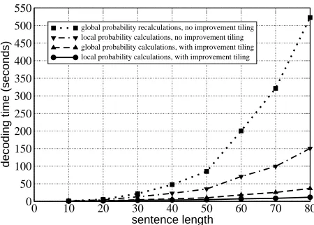
Figure 2: Runtimes for sentences of length 10–80. The

graph shows the average runtimes ( ) of 10 different

sample sentences of the respective length with swap op-erations restricted to a maximum swap segment size of 5 and a maximum swap distance of 2.

. The original algorithm pursues a highly

in-efficient search strategy. At the end of each iteration, only the single best improvement is executed; all others, even when independent, are discarded. In other words, the al-gorithm needs one search iteration per improvement. We assume that there is a linear correlation between input length and the number of improvements — an assump-tion that is supported by the empirical data in Fig. 4.

Therefore,

.

( , restricted swapping)

( , restricted swapping)

(no restrictions on swapping).

The number of search steps per iteration is the sum of the number of search steps for CHANGE, SWAP, JOIN, INSERT, and ERASE. The highest order term in this sum is unrestricted SWAP with

.

With restricted swapping, S has a theoretical complex-ity of

(due to JOIN) in decoding, but the

con-tribution of the JOIN operation to overall time consump-tion is so small that it can be ignored for all practical

pur-poses. Therefore, the average complexity of in practice

is

, and the total complexity of in practice is

-/.

L

.

J

D . 3 50

In decoding, which combines up to two CHANGE

operations or one CHANGE operation and one INSERT

operation, has a practical complexity of

, so that

-/.

L

.

J

D

. . E

.

We discuss below how can be reduced to practically

linear time for decoding as well.

4

Reducting Decoder Complexity

Every change to the alignment affects only a few of the individual probabilities that make up the overall align-ment score: the n-gram contexts of those places in the English hypothesis where a change occurs, plus a few translation model probabilities. We call the — not neces-sarily contiguous — area of an alignment that is affected by a change the change’s local context.

With respect to an efficient implementation of the greedy search, we can exploit the notion of local con-texts in two ways. First, we can limit probability recal-culations to the local context (that is, those probabilities that actually are affected by the respective change), and secondly, we can develop the notion of change

dependen-cies: Two changes are independent if their local contexts

do not overlap. As we will explain below, we can use this notion to devise a scheme of improvement caching

and tiling (ICT) that greatly reduces the total number of

alignments considered during the search.

Our argument is that local probability calculations and ICT each reduce the complexity of the algorithm by

prac-tically

, that is, from

to

/

with .

Thus, the complexity for decreases from

43

to

. If we limit the search space for the second

oper-ation (CHANGE or INSERT) in decoding to its

lo-cal context, decoding, too, has practically linear

com-plexity, even though with a much higher coefficient (cf Fig. 6).

4.1 Local Probability Calculations

The complexity of calculating the alignment

probabil-ity globally (that is, over the entire alignment) is

.

However, since there is a constant upper bound3 _{on the}

size of local contexts,

EDFHGIKJF

needs to be performed only once for the initial gloss, therafter, recalculation of only those probabilities affected by each change (

FHGLMJF

) suffices. This reduces the overall decoding com-plexity from

to

/

with .

Even though profoundly trivial, this improvement sig-nificantly reduces translation times, especially when im-provements are not tiled (cf. below and Fig. 2).

4.2 Improvement Caching and Tiling4_(ICT)

Based on the notions of local contexts and change depen-dencies, we devised the following scheme of

improve-ment caching and tiling (ICT): During the search, we

keep track of the best possible change affecting each local context. (In practice, we maintain a map that maps from

3

In practice, 16 with a trigram language model: a swap of two large segments over a large distance affects four points in

the English hypothesis, resulting in 7 trigrams, plus

four individual distortion probabilities.

4

initial gloss us localities computer system suffer computer virus attack and refused service attack and there various security loopholes instance everywhere

alignments checked: 1430

possible improvements: 28

improvements applied: 5

u.s. localities computer system opposed computer virus attack and rejecting service

attack and there are various security loopholes instance everywhere .

alignments checked: 1541

possible improvements: 3

improvements applied: 3

u.s. citizens computer system opposed the computer virus attack and rejecting service

attack and there are various security loopholes publicize everywhere .

alignments checked: 768

possible improvements: 1

improvements applied: 1

u.s. citizens computer system opposed to the computer virus attack and rejecting service attack and there are various security loopholes publicize everywhere .

alignments checked: 364

possible improvements: 1

improvements applied: 1

u.s. citizens computer system is opposed to the computer virus attack and rejecting service attack and there are various security loopholes publicize everywhere .

alignments checked: 343

possible improvements: 0

improvements applied: 0

u.s. citizens computer system is opposed to the computer virus attack and rejecting service attack and there are various security loopholes publicize everywhere .

Figure 3: A decoding trace using improvement caching and tiling (ICT). The search in the second and later iterations is limited to areas where a change has been applied (marked in bold print) — note that the number of alignment checked goes down over time. The higher number of alignments checked in the second iteration is due to the insertion of an additional word, which increases the number of possible swap and insertion operations. Decoding without ICT results in the same translation but requires 11 iterations and checks a total of 17701 alignments as opposed to 5 iterations with a total of 4464 alignments with caching.

the local context of each change that has been considered to the best change possible that affects exactly this

con-text.) At the end of the search iteration @

, we apply a very restricted stack search to find a good tiling of non-overlapping changes, all of which are applied. The goal of this stack search is to find a tiling that maximizes the overal gain in alignment probability. Possible improve-ments that overlap with higher-scoring ones are ignored. In the following search iteration

@ $

, we restrict the

search to changes that overlap with changes just applied. We can safely assume that there are no improvements to be found that are independent of the changes applied at the end of iteration

@

: If there were such improvements, they would have been found in and applied after iteration

@

. Figure 3 illustrates the procedure.

We assume that improvements are, on average, evenly distributed over the input text. Therefore, we can expect the number of places where improvements can be applied to grow with the input length at the same rate as the num-ber of improvements. Without ICT, the numnum-ber of iter-ations grows linearly with the input length, as shown in Fig. 4. With ICT, we can parallelize the improvement process and thus reduce the number of iterations for each search to a constant upper bound, which will be deter-mined by the average ‘improvement density’ of the do-main. One exception to this rule should be noted: since the expected number of spurious words (words with no counterpart in English) in the input is a function of the

input length, and since all changes in word translation that involve the NULL word are mutually dependent, we should expect to find a very weak effect of this on the number of search iterations. Indeed, the scatter diagram in Fig.4 suggests a slight increase in the number of

itera-tions as the input length increases.5

At the same time, however, the number of changes con-sidered during each search iteration eventually decreases, because subsequent search iterations are limited to areas where a change was previously performed. Empirical ev-idence as plotted on the right in Fig. 4 suggests that this effect “neutralizes” the increase in iterations in depen-dence of the input length: the total number of changes considered indeed appears to grow linearly with the in-put length. It should be noted that ICT, while it does change the course of the search, primarily avoids re-dundant search steps — it does not necessarily search a smaller search space, but searches it only once. The to-tal number of improvements found is roughly the same (15,299 with ICT, 14,879 without for the entire test cor-pus with a maximum swap distance of 2 and a maximum swap segment size of 5).

5

0 10 20 30 40 50 60 70 80 90 100 input length (in words/tokens)

0 10 20 30 40 50 60 70 80

number of search iterations

without improvement caching and tiling with improvement caching and tiling

0 10 20 30 40 50 60 70 80 90 100

input length (in words/tokens) 0

250 500 750 1000 1250 1500 1750

number of hypotheses checked (in thousand)

without improvement caching and tiling with improvement caching and tiling

Figure 4: Number of search iterations (left) and total number of alignments considered (right) during search in depen-dence of input length. The data is taken from the translation of the Chinese testset from the TIDES MT evaluation in June 2002. Translations were performed with a maximum swap distance of 2 and a maximum swap segment size of 5.

4.3 Restrictions on Word Reordering

With

, unlimited swapping swapping is by far the biggest consumer of processing time during decoding. When translating the Chinese test corpus from the 2002

TIDES MT evaluation6without any limitations on

swap-ping, swapping operations account for over 98% of the total search steps but for less than 5% of the improve-ments; the total translation time (with ICT) is about 34 CPU hours. For comparison, translating with a maximum swap segment size of 5 and a maximum swap distance of 2 takes ca. 40 minutes under otherwise unchanged cir-cumstances.

It should be mentioned that in practice, it is generally not a good idea to run the decoder with without restric-tions on swapping. In order to cope with hardware and time limitations, the sentences in the training data are typ-ically limited in length. For example, the models used for the experiments reported here were trained on data with a sentence length limit of 40. Sentence pairs where one of the sentences exceeded this limit were ignored in train-ing. Therefore, any swap that involves a distortion greater than that limit will result in the minimal (smoothed) dis-tortion probability and most likely not lead to an improve-ment. The question is: How much swapping is enough? Is there any benefit to it at all? This is an interesting ques-tion since virtually all efficient MT decoders (e.g. Till-mann and Ney, 2000; Berger et al., 1994; Alshawi et al., 2000; Vidal, 1997) impose limits on word reordering.

In order to determine the effect of swap restrictions on decoder performance, we translated the Chinese test cor-pus 101 times with restrictions on the maximum swap

6

100 short news texts; 878 text segments; ca. 25K

to-kens/words.

0 1 2 3 4 5 6 7 8 9 10

maximum swap distance

0 1

2 3

4 5

6 7

8 9

10

maximum swap segment size 0.138

0.139 0.140 0.141 0.142 0.143 0.144 0.145

BLEU score

Figure 5: BLEUscores for the Chinese test set (

de-coding) in dependence of maximum swap distance and maximum swap segment size.

distance (MSD) and the maximum swap segment size (MSSS) ranging from 0 to 10 and evaluated the

transla-tions with the BLEU7_{metric (Papineni et al., 2002). The}

results are plotted in Fig. 5.

On the one hand, the plot seems to paint a pretty clear picture on the low end: score improvements are compar-atively large initially but level off quickly. Furthermore, the slight slope suggests slow but continuous improve-ments as swap restrictions are eased. For the Arabic test data from the same evaluation, we obtained a sim-ilar shape (although with a roughly level plateau). On the other hand, the ‘bumpiness’ of the surface raises the question as to which of these differences are statistically

7

Table 1: Decoder performance on the June 2002 TIDES MT evluation test set with multiple searches from randomized starting points (MSD=2, MSSS=5).

default 2 searchesbest of 3 searchesbest of 4 searchesbest of 5 searchesbest of 6 searchesbest of 7 searchesbest of 8 searchesbest of 9 searchesbest of 10 searchesbest of 11 searchesbest of

G1 BLEU 0.143 0.145 0.146 0.148 0.148 0.150 0.150 0.150 0.150 0.150 0.151

RSER* 93.7% 91.8% 89.8% 87.7% 86.1% 85.2% 83.9% 82.1% 81.2% 80.1% 77.9%

G2 BLEU 0.145 0.150 0.151 0.151 0.154 0.154 0.154 0.154 0.154 0.155 0.156

RSER 77.2% 69.1% 61.2% 55.0% 48.3% 42.5% 36.6% 30.5% 23.9% 20.0% 13.6%

* RSER = relative search error rate; percentage output sentences with suboptimal alignment probability

significant.

We are aware of several ways to determine the statisti-cal significance of BLEU score differences. One is

boot-strap resampling (Efron and Tibshirani, 1993)8_to

deter-mine confidence intervals, another one splitting the test corpus into a certain number of subcorpora (e.g. 30) and then using the t-test to compare the average scores over these subcorpora (cf. Papineni et al., 2001). Bootstrap resampling for the various system outputs leads to very similar confidence intervals of about 0.006 to 0.007 for a one-sided test at a confidence level of .95. With the t-score method, differences in score of 0.008 or higher seem to be significant at the same level of confidence. According to these metrics, none of the differences in the plot are significant, although the shape of the plot sug-gests that moderate swapping probably is a good idea.

In addition to limitations of the accuracy of the BLEU method itself, variance in the decoders performance can blur the picture. A third method to determine a confi-dence corridor is therefore to perform several random-ized searches and compare their performance. Follow-ing a suggestion by Franz Josef Och (personal commu-nications), we ran the decoder multiple times from ran-domized starting glosses for each sentence and then used the highest scoring one as the “official” system output. This gives us a lower bound on the price in performance that we pay for search errors. The results for up to ten searches from randomized starting points in addition to the baseline gloss are given in Tab. 1. Starting points were randomized by randomly picking one of the top 10 translation candidates (instead of the top candidate) for each input word, and performing a (small) random num-ber of SWAP and INSERT operations before the actual search started. In order to insure consistency across re-peated runs, we used a pseudo random function. In our

experiments, we did not mix and decoding. The

practical reason for this is that decoding takes more

than ten times as long as decoding. As the table

illus-trates, running multiple searches in from randomized

starting points is more efficient that running once.

8

Thanks to Franz Josef Och for pointing this option out to us.

Choosing the best sentences from all decoder runs results in a BLEU score of 0.157. Interestingly, the decoding time from the default starting point is much lower (G1: ca. 40 min. vs. ca. 1 hour; G2: ca. 9.5 hours vs. ca. 11.3 hours), and the score, on average, is higher than when searching from a random starting point (G1: 0.143 vs. 0.127 (average); G2: 0.145 vs. 0.139 (average)). This indicates that the default seeding strategy is a good one.

From the results of our experiments we conclude the following.

First, Tab. 1 suggests that there is a good correla-tion between IBM Model 4 scores and the BLEU met-ric. Higher alignment probabilities lead to higher BLEU

scores. Even though hardly any of the score

differ-ences are statistically significant (see confidence intervals above), there seems to be a trend.

Secondly, from the swapping experiment we conclude that except for very local word reorderings, neither the IBM models nor the BLEU metric are able to recognize long distance dependencies (such as, for example, ac-counting for fundamental word order differences when translating from a SOV language into a SVO language). This is hardly surprising, since both the language model for decoding and the BLEU metric rely exclusively on n-grams. This explains why swapping helps so little. For a different approach that is based on dependency tree trans-formations, see Alshawi et al. (2000).

Thirdly, the results of our experiments with random-ized searches show that greedy decoding does not per-form as well on longer sentences as one might conclude from the findings in Germann et al. (2001). At the same time, the speed improvements presented in this paper make multiple searches feasible, allowing for an overall faster and better decoder.

5

Conclusions

In this paper, we have analyzed the complexity of the greedy decoding algorithm originally presented in Ger-mann et al. (2001) and presented improvements that dras-tically reduce the decoder’s complexity and speed to practically linear time.

10 20 30 40 50 60 70 80

sentence length

0 1 2 3 4 5 6 7 8 9 10 11

average time consumption (in sec.)

G1 decoding

SWAP CHANGE

INSERT JOIN

10 20 30 40 50 60 70 80

sentence length

0 10 20 30 40 50 60 70 80 90 100 110 120 130 140 150 160 170

average time consumption (in sec.)

G2 decoding

SWAP CHANGE INSERT

G1 total decoding time

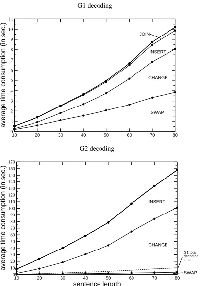
Figure 6: Time consumption of the various change types in

7 and decoding (with 10 translations per input word

con-sidered, a list of 498 candidates for INSERT, a maximum swap distance of 2 and a maximum swap segment size of 5). The pro-files shown are cumulative, so that the top curve reflects the total decoding time. To put the times for decoding in perspective,

the dashed line in the lower plot reflects the total decoding time in 7 decoding. Operations not included in the figures consume

so little time that their plots cannot be discerned in the graphs. The times shown are averages of 100 sentences each for length 10, 20, , 80.

IBM Model 4 scores and the BLEU metric. The speed improvements discussed in this paper make multiple ran-domized searches per sentence feasible, leading to a faster and better decoder for machine translation with IBM Model 4.

6

Acknowledgements

We are very grateful to Franz Josef Och for various very helpful comments on the work reported in this paper. This work was supported by DARPA-ITO grant N66001-00-1-9814.

References

Alshawi, Hiyan, Douglas, Shona, and Bangalore, Srini-vas. 2000. Learning dependency translation models as collections of finite-state head transducers.

Computa-tional Linguistics, 26(1):45–60.

Berger, Adam L., Brown, Peter F., Della Pietra, Stephen A., Della Pietra, Vincent J., Gillet, John R.,

Lafferty, John D., Mercer, Robert L., Printz, Harry, and Ureˇs, Luboˇs. 1994. The candide system for machine translation. In: Proceedings of the Arpa Workshop on

Human Language Technology.

Berger, Adam L., Brown, Peter F., Della Pietra, Stephen A., Della Pietra, Vincent J., Kehler, An-drew S., and Mercer, Robert L. 1996. Language lation apparatus and method using context-based trans-lation models. United States Patent 5,510,981.

Brown, Peter F., Cocke, John, Della Pietra, Stephen A., Della Pietra, Vincent J., Jelinek, Fredrick, Lafferty, John D., Mercer, Robert L., and Roossin, Paul S. 1990. A statistical approach to machine translation.

Compu-tational Linguistics, 16(2):79–85.

Brown, Peter F., Della Pietra, Vincent J., Della Pietra, Stephen A., and Mercer, Robert L. 1993. The mathe-matics of statistical machine translation: Parameter es-timation. Computational Linguistics, 19(2):263–311.

Efron, Bradley and Tibshirani, Robert J. 1993. An

Intro-duction to the Bootstrap. Chapman & Hall/CRC.

Germann, Ulrich, Jahr, Michael, Knight, Kevin, Marcu, Daniel, and Yamada, Kenji. 2001. Fast decoding and optimal decoding for machine translation. In:

Proceed-ings of the 39th ACL. Toulouse, France, 228–235.

Knight, Kevin. 1999. Decoding complexity in

word-replacement translation models. Computational

Lin-guistics, 25(4):607–615.

Och, Franz Josef, Ueffing, Nicola, and Ney, Hermann. 2001. An efficient A* search algorithm for statistical machine translation. In: Proceedings of the ACL 2001

Workshop on Data-Driven Methods in Machine Trans-lation. Toulouse, France, 55–62.

Papineni, Kishore, Roukos, Salim, Ward, Todd, and Zhu, Wei-Jing. 2002. Bleu: a method for automatic eval-uation of machine translation. In: Proceedings of the

40th ACL. Philadelphia, PA, 311–318.

Papineni, Kishore, Roukos, Salim, Ward, Tood, and Zhu, Wei-Jing. 2001. Bleu: a method for automatic eval-uation of machine translation. Tech. Rep. RC22176 (W0109-022), IBM Research Division, Thomas J. Watson Research Center.

Tillmann, Christoph and Ney, Hermann. 2000. Word re-ordering and DP-based search in statistical machine

translation. In: Proceedings of the 18th COLING.

Saarbr¨ucken, Germany, 850–856.

Vidal, Enrique. 1997. Finite-state speech-to-speech trans-lation. In: Proceedings of the 22nd ICASSP. Munich, Germany, 111–114.

Wang, Ye-Yi and Waibel, Alex. 1997. Decoding algo-rithm in statistical machine translation. In: