985
Spider-Jerusalem at SemEval-2019 Task 4: Hyperpartisan News Detection
Amal Alabdulkarim
Department of Computer Science Columbia University [email protected]
Tariq Alhindi
Department of Computer Science Columbia University [email protected]
Abstract
This paper describes our system for detecting hyperpartisan news articles, which was submitted for the shared task in SemEval 2019 on Hyperpartisan News Detection. We developed a Support Vector Machine (SVM) model that uses TF-IDF of tokens, Language Inquiry and Word Count (LIWC) features, and structural features such as number of paragraphs and hyperlink count in an article. The model was trained on 645 articles from two classes: mainstream and hyperpartisan. Our system was ranked seventeenth out of forty two participating teams in the binary classification task with an accuracy score of 0.742 on the blind test set (the accuracy of the top ranked system was 0.822). We provide a detailed description of our preprocessing steps, discussion of our experiments using different combinations of features, and analysis of our results and prediction errors.
1 Introduction
Fake news on various online media outlets misinform the public and threaten the integrity of journalism. This has serious effects on shaping public opinions on controversial topics such as climate change, and swaying voters in political elections. Yellow press existed long before the digital age but had limited reach when compared to mainstream press. However, with the introduction of social media, news that are extremely biased (hyperpartisan) tend to spread more quickly than the ones that are not (Vosoughi et al., 2018). Therefore, there is a need for automatic detection methods of hyperpartisan news. Computational methods for fighting fake news mainly focus on automatic fact-checking rather than looking at writing styles of news articles (Potthast et al., 2018). SemEval-2019 Hyperpartisan News Detection shared task aims to study the ability of a system to detect if a given article exhibits a hyperpartisan argumentation
writing style to convince readers of a certain position. The shared task introduces a binary classification task of classifying an article into one of two possibilities: mainstream or hyperpartisan. The data for the shared task was introduced by (Kiesel et al.,2019) and consists of 645 of articles from mainstream, left-wing, and right-wing publishers. The articles from both left-wing and right-wing publishers were labeled as hyperpartisan.
The baseline system to detect hyperpartisan developed by (Potthast et al., 2018) uses Unmasking (Koppel et al.,2007) and was trained on 1,627 of articles. The articles are from nine publishers in the US: three mainstream (ABC News, CNN, and Politico), three left-wing (Addicting Info, Occupy Democrats, and The Other 98%), and three right-wing (Eagle Rising, Freedom Daily, and Right Wing News). Their model had a best accuracy of 75% by using stylistic features. However, their model is not directly comparable with ours since the dataset for the shared task is different.
In the following sections, we describe our system for identifying hyperpartisan news articles as part of our participation in the Hyperpartisan New Detection shared task in SemEval 2019 (Kiesel et al.,2019).
2 System Description
We trained a support vector machine model on a feature vector representing each article in our training dataset. To develop this model, we processed the dataset and analyzed different features and feature combinations.
2.1 Pre-processing
We clean the articles and titles from punctuation marks, stop words, none alphabetical characters, lemmatized and tokenized using the Natural Language Toolkit (NLTK) (Bird et al., 2009) . After that, those tokens are processed using the TF-IDF vectorizer in sci-kit-learn (Pedregosa et al.,2011) and stored as a vector.
2.2 Feature Extraction
The features we chose to extract from the articles, include the following:
1. Words vector. After pre-processing all the unigrams in the articles and the titles are stored in a TF-IDF vector.
2. Linguistic Inquiry and Word Count (LIWC) features. The words in every article and titles that are part of any dimension of the Linguistic Inquiry and Word Count (LIWC) dictionary. LIWC analyzes text by using a dictionary of the most common words and word stems. The dictionary is organized into different categories, some of which are affect words and function words. (Pennebaker et al., 2012) are counted and stored in a sixty-three dimensional TF-IDF vector.
3. Punctuation. The punctuation marks in the title and articles were grouped into six different categories and then counted and stored separately from the article and then stored in a six-dimensional TF-IDF vector. Because we were specifically interested in exclamation marks, question marks and quotations we let those three punctuation marks have their independent counts in the vector. The other three dimensions are colons and comma, dot, and parenthesis.
4. Article structure features:Paragraphs, quotes, and external links are counted and stored in a 3-dimensional vector.
5. Emotion features. The emotional content in the articles is captured using the NRC emotions lexicon (Mohammad and Turney, 2013). After counting the words in each emotion category, we store the counts in a ten-dimensional vector, where the elements represent anger, anticipation, disgust, fear, joy, negative, positive, sadness, surprise and trust.
After pre-processing and extraction, we experiment with different groupings of these features in our model to see which group of features is most effective for the given task. The next section discusses those feature combinations.
Features Title Article F1
W L P E W L P E S
1 x x x x 0.48
2 x x x x 0.75
3 x x x x x 0.74
4 x x x x x x x x x 0.72
5 x x 0.76
6 x x x x x x x 0.71
7 x x x x 0.76
8 x x x x x x 0.74
9 x x 0.48
10 x x 0.48
11 x x 0.70
[image:2.595.310.526.139.307.2]12 x x x x x 0.76
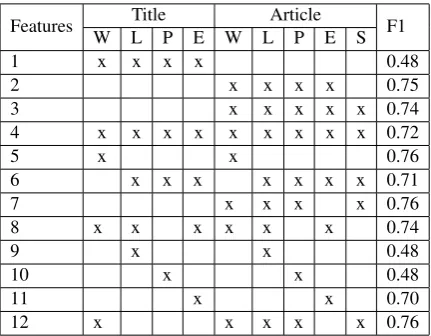
Table 1: Different feature combinations (W: Words vector, L: LIWC features, P: Punctuation Marks, E: Emotions and S: Articles Structure) and their weighted F1 score on the local validation set.
2.3 Feature Selection
Now that we have the extracted features we began grouping them and testing them in our model. We tested the different combinations of these features as shown in Table 1. In these experiments, the most effective combination of features was number 7 (the word tokens, LIWC, punctuation marks, and the article structure), number 5 (the word tokens of the article and title) and number 12 (all the features in 5 and 7). The other title features did not provide a good contribution to the model as we expected.
2.4 Model
The model1 is constructed using a sci-kit-learn pipeline with two main steps. The first part is a dimensionality reduction using latent semantic indexing (Manning et al.,2008) using Truncated Singular value decomposition (SVD). The primary goal of using an SVD is to lower the rank of the feature matrix by merging the dimensions associated with terms that have a similar meaning. The second step is a linear support vector machine (SVM) model used in default settings, which takes as input the output of the
1
SVD. The SVM is useful in high dimensional spaces and when the number of features is higher than the number of articles in the dataset.
3 Results
In this section, we will review the results of our model and show its performance on a local validation set of size 129 articles (48 hyperpartisan, 81 not hyperpartisan) and the test set on TIRA (Potthast et al.,2019).
Measure Validation Set Test Set
accuracy 0.767 0.742
f1-score 0.767 0.709
precision 0.767 0.814
recall 0.767 0.627
true positives 26 197
true negatives 73 269
false positives 8 45
[image:3.595.82.282.218.346.2]false negatives 22 117
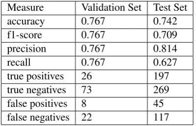
Table 2: Main task classification results of the local validation and test datasets.
3.1 Main Task
For the main task, identifying hyperpartisan articles from a dataset of manually labeled articles, we created a local validation set, by partitioning the by-article dataset into a training and validation sets while keeping the split ratio equal in both. We do not report any results on the by-publisher datatset as we found class mismatch for some articles across the two datasets (i.e. some articles are labeled mainstream in the by-article and hyperpartisan in the by-publisher). Therefore, we decided to focus on the more accurately labeled dataset (the by-article), which is also the one used for share-task leaderboard ranking.
Model Accuracy
validation set test set
SVM 0.767 0.742
Ensemble 0.829 0.640
Ensemble-RNN 0.76* 0.694
Table 3: Classification results of various models. Ensemble-RNN model was tested using cross-validation so it is not directly comparable with the other two models in the validation scores.
In Table 2, we show the classification report of the SVM model after running on a local validation set and the official test set. When we tested the SVM model locally, it gave a high f1-score 0.767 which is the measure we relied on locally because the data was not balanced. On the task leaderboard, tested on the test set in TIRA, the model ranked 17 among the 42 participating teams, with an accuracy of 0.742.
We also experimented with other machine learning models and compared them with our SVM model. We developed an ensemble model that consists of an SVM classifier, a Gradient Boosting Classifier and a Bagging Classifier with a decision tree as its base estimator. But that classifier only scored 0.64 accuracy on the test set, even though it scored 0.829 accuracy on the validation set. We also added an RNN classifier that uses ELMO embeddings (Peters et al.,2018) to the previously described ensemble model. That model increased the accuracy on the test set by a small value 0.694 but did not outperformed the SVM model.
3.2 Meta Learning
We also participated in the meta-learning sub-task, the task is to use all of the predictions from all of the participating teams classifiers as an input and come up with a meta classifier.
The dataset we were given is a list of predictions from all the participating classifiers and the gold labels for each article in this list. The model we developed builds on the idea of a weighted majority algorithm but with changes to how the weights are being calculated. So instead of dividing by the total number of elements to calculate the weights, we have two separate weights, one for each class, and then we calculated those two weights for each classifier using equation 1 where H in the equation corresponds to the class (0 or 1), c is the classifier and y is the true label.
w(c, H) = Pn
i 1(y=H∧c(x) =H)
Pn
i 1(y ==H)
(1)
[image:3.595.84.282.634.704.2]4 Discussion
We can observe from the results in Table 1 that the TF-IDF features of articles and titles are the most useful for this task. They consistently have the highest accuracy score when combined with other features or when used alone as shown in feature set 5 in Table 1. This shows that it was hard for LIWC features by themselves to capture any linguistic patterns that correlate with hyperpartisan news. The superiority of TF-IDF could be due to trends related to a certain domain or publisher rather than to a general hyperpartisan trend. In order to examine the ability of other approaches to detect hyperpartisan news articles, we developed two other models. An Ensemble model of three models and an Ensemble-RNN model both described in Section 3.1. Both models scored almost as good as the SVM on the validation set (Ensemble-RNN model) or better than the SVM (Ensemble model). However, both scored significantly lower than the SVM model on the blind test set. The Ensemble-RNN model included a neural network which was trained on our small training set of 645 articles. Given the huge drop between validation and test scores, especially for the ensemble mode which dropped from 0.83 to 0.64, this indicates an overfitting on the training data. Although the deep learning models were not trained for more than five epochs to avoid overfitting, they were not able to learn beyond what was seen in the training data and were possibly memorizing the data. The complexity and subjectivity of the annotation task could have made it harder for the model to classify articles. We were also dealing with imbalance class sizes which made the model learn to predict one class better than the other. As for the meta-learning experiment, we followed a class-based weighted majority approach, where the classifiers that are better in classification of one class were given a higher weight for that class predictions and lower weight for their predictions in the other class. However, this approach only had a one-point improvement over the baseline. We analyzed the prediction errors of the SVM model to further understand what causes the model to make a wrong prediction.
4.1 Error Analysis
We looked more closely at four examples: one correct and one wrong prediction from each class.
The first example is an article from Fox News about the 2016 US presidential elections 2. This article was labeled as mainstream and was predicted correctly by our model. Although the article was predicted correctly by the classifier, it was not clear to us why this article was labeled as mainstream as it has a somewhat one-sided view to its story and thus could be labeled as hyperpartisan. This points out the uncertainty or noise in the annotation of some data points. The second mainstream article is from Yahoo! news and talks about Ivanka Trump3. It was wrongly classified as hyperpartisan by our model. This could be due to the fact that the content of the article is related to Trump, which appeared more in the hyperpartisan class in our dataset. The third article is labeled as hyperpartisan and predicted as such. It is an opinion piece from Online Athens about social justice 4. It has phrases such as “so-called” and “Karl Marx would be so proud” which could’ve helped the model to use the learned TF-IDF features of the training data to make a correct prediction. The final article we looked at is from Real Clear Politics and talks about a joke made by Jimmy Kimmel5. This was wrongly classified as mainstream by the model which could be due to having structural features of mainstream articles (long article and no URLs). These four examples show that some of our lexical and structural features did not generalize well to the test set.
5 Conclusion
We presented an SVM model that detects hyperpartisan news articles with a 0.742 accuracy after it was trained on a total 645 articles from mainstream and hyperpartisan classes. This task was primarily challenging due to the complexity in labeling such articles, and differences in writing styles across domains, publishers and individuals. The small size of the training data along with the class imbalance also contributed to the complexity, which made it harder for the model to learn. We presented a summary of our experiments and analysis of our results and prediction errors.
2http://insider.foxnews.com/2016/10/14/ 3
http://www.yahoo.com/news/truck-ad-featuring-ivanka
4
http://onlineathens.com/opinion/2017-10-19/
References
Steven Bird, Ewan Klein, and Edward Loper. 2009. Natural Language Processing with Python. O’Reilly Media, Inc.
Johannes Kiesel, Maria Mestre, Rishabh Shukla, Emmanuel Vincent, Payam Adineh, David Corney, Benno Stein, and Martin Potthast. 2019. SemEval-2019 Task 4: Hyperpartisan News Detection. Proceedings of The 13th International Workshop on Semantic Evaluation (SemEval 2019).
Johannes Kiesel, Maria Mestre, Rishabh Shukla, Emmanuel Vincent, David Corney, Payam Adineh, Benno Stein, and Martin Potthast. 2018. Data for PAN at SemEval 2019 Task 4: Hyperpartisan News Detection.
Moshe Koppel, Jonathan Schler, and Elisheva Bonchek-Dokow. 2007. Measuring Differentiability: Unmasking Pseudonymous Authors. Journal of Machine Learning Research, (8):1261–1276.
Christopher D. Manning, Prabhakar. Raghavan, and Hinrich. Schutze. 2008. Introduction to information retrieval. Cambridge University Press.
Saif M Mohammad and Peter D Turney. 2013. Crowdsourcing a Word-Emotion Association Lexicon.Computational Intelligence, 29:436–465.
Fabian Pedregosa, Vincent Michel, Olivier Grisel OLIVIERGRISEL, Mathieu Blondel, Peter Prettenhofer, Ron Weiss, Jake Vanderplas, David Cournapeau, Gal Varoquaux, Alexandre Gramfort, Bertrand Thirion, Olivier Grisel, Vincent Dubourg, Alexandre Passos, Matthieu Brucher, Matthieu Perrot and ´Edouardand, Anddouard Duchesnay, and FRdouard Duchesnay EDOUARDDUCHESNAY. 2011. Scikit-learn: Machine Learning in Python Ga¨el Varoquaux Bertrand Thirion Vincent Dubourg Alexandre Passos PEDREGOSA, VAROQUAUX, GRAMFORT ET AL. Matthieu Perrot. Technical report, Parietal, INRIA Saclay.
James W Pennebaker, Roger J Booth, Ryan L Boyd, and Martha E Francis. 2012. Linguistic Inquiry and Word Count: LIWC2015 Operator’s Manual. In Applied Natural Language Processing, pages 206– 229. IGI Global.
Matthew E. Peters, Mark Neumann, Mohit Iyyer, Matt Gardner, Christopher Clark, Kenton Lee, and Luke Zettlemoyer. 2018. Deep contextualized word representations.
Martin Potthast, Tim Gollub, Matti Wiegmann, and Benno Stein. 2019. TIRA Integrated Research Architecture. InInformation Retrieval Evaluation in a Changing World - Lessons Learned from 20 Years of CLEF. Springer.
Martin Potthast, Johannes Kiesel, Kevin Reinartz, Janek Bevendorff, and Benno Stein. 2018. A
Stylometric Inquiry into Hyperpartisan and Fake News. 56th Annual Meeting of the Association for Computational Linguistics (ACL 2018), page 231240.