LEABHARLANN CHOLAISTE NA TRIONOIDE, BAILE ATHA CLIATH TRINITY COLLEGE LIBRARY DUBLIN OUscoil Atha Cliath The University of Dublin
Terms and Conditions of Use of Digitised Theses from Trinity College Library Dublin
Copyright statement
All material supplied by Trinity College Library is protected by copyright (under the Copyright and Related Rights Act, 2000 as amended) and other relevant Intellectual Property Rights. By accessing and using a Digitised Thesis from Trinity College Library you acknowledge that all Intellectual Property Rights in any Works supplied are the sole and exclusive property of the copyright and/or other I PR holder. Specific copyright holders may not be explicitly identified. Use of materials from other sources within a thesis should not be construed as a claim over them.
A non-exclusive, non-transferable licence is hereby granted to those using or reproducing, in whole or in part, the material for valid purposes, providing the copyright owners are acknowledged using the normal conventions. Where specific permission to use material is required, this is identified and such permission must be sought from the copyright holder or agency cited.
Liability statement
By using a Digitised Thesis, I accept that Trinity College Dublin bears no legal responsibility for the accuracy, legality or comprehensiveness of materials contained within the thesis, and that Trinity College Dublin accepts no liability for indirect, consequential, or incidental, damages or losses arising from use of the thesis for whatever reason. Information located in a thesis may be subject to specific use constraints, details of which may not be explicitly described. It is the responsibility of potential and actual users to be aware of such constraints and to abide by them. By making use of material from a digitised thesis, you accept these copyright and disclaimer provisions. Where it is brought to the attention of Trinity College Library that there may be a breach of copyright or other restraint, it is the policy to withdraw or take down access to a thesis while the issue is being resolved.
Access Agreement
By using a Digitised Thesis from Trinity College Library you are bound by the following Terms & Conditions. Please read them carefully.
Microphone array techniques for aeroacoustics
Peter Jordan
Department o f Mechanical Engineering,
Trinity College,
Dublin
October 2000
A b stract
The capacity for source localisation and measurement in aeroacoustics can be
enhanced through the use of a microphone array. Although arrays have been
used in a variety of applications, there are a number of problems manifest
in their use for analysis of specific systems. The first of these is the depen
dence of the response characteristic of an array on the source frequency of the
system being analysed. This can lead both to spurious source identification
and erroneous source measurement. In this work a technique developed for
radio antenna applications is adapted to give additional response control for
linear arrays with commensurate element spacing. This is then applied to an
aeroacoustic system consisting of twin high-speed propellers where the noise
generated by one propeller is to measured, while contributions from the other
are filtered out. The second problem arises due to aeroacoustic source direc
tivity. This problem is illustrated by means of a simple model, which shows
th a t erroneous results are obtained when a dipole source is measured using an
ordinary beamformer. A procedure which allows the location and orientation
of such a source to be identified is proposed, and a correction applied to the
beamformer such th a t it correctly measures the source. This procedure is then
applied to an experimental aeroacoustic system containing a single dipole in
the form of a cylinder in cross-flow. A general methodology for aeroacous
tic analysis based on these developments is proposed and its implementation
T I4-4- I
j I
' ' = — ^
— ft-TTfg
i r ^ r ^
,1. .♦?- £ , t7 - = r ^ ^ 7 J> i . T |
( i Z i
- " i i
r 1 1 f f
-r"*rr*^
u
I
r r 1 r r
J? " ^
( ii
ffP o e o grandtoto
,0,1.
1:
e;
i|
uj
1
y
.
i
Il
f.
-
;
S
L
1
-- -- -- -- ~p p T ~
^
^ f -p
Declaration
I declare that I am the sole author o f this thesis and that all the work presented in
it, unless otherwise referenced, is my own. I also declare that this work has not
been submitted, in whole or in part, to any other university or college for any
degree or other qualification.
I authorise the library o f the University o f Dublin to lend this thesis.
Acknowledgements
C on ten ts
1
In tro d u ctio n
1
1.1
Engineering and noise ...
1
1.1.1 Aeroacoustic noise ...
2
1.1.2 Reducing noise le v e ls ...
3
1.2
The microphone a r r a y ...
3
2
R e v ie w o f array tech n iq u es
5
2.1
Historical p ersp e c tiv e...
5
2.2
Beamforming and some of its p r o b le m s ...
10
2.2.1 D irectiv ity ...
11
2.2.2 Source localisation in acoustics and aeroacoustics . . .
14
2.2.3 Microwave antennae
...
16
2.3 S u m m a r y ...
17
3
D ir e c tiv ity m od ellin g and control
20
3.1
In tro d u c tio n ...
20
3.2
Near field formulation of array response...
20
3.3
Far field formulation of array response ...
23
3.4
Application of Schelkunoff’s t h e o r y ...
26
3.4.1 Directivity c o m p a riso n ...
26
3.5 A case s tu d y ...
28
3.5.3
The cross a r r a y ... .
33
3.5.4 The circular a r r a y ...
33
3.6
D isc u ssio n ...
37
3.7
C onclusion...
40
4 A pplication to aeroacoustics
43
4.1
In tro d u c tio n ...
43
4.1.1 The m on o pole...
43
4.1.2 The d ip o le ...
44
4.1.3 The q u a d ru p o le ...
46
4.1.4 Summary of source characteristics...
47
4.2 Source identification in a e ro a c o u s tic s ...
48
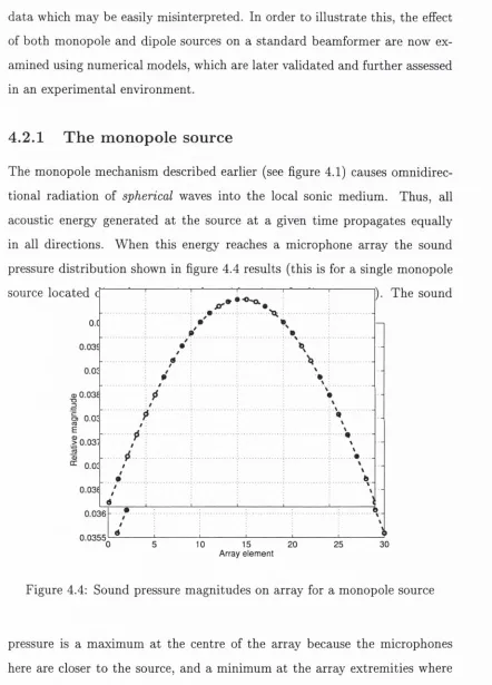
4.2.1 The monopole s o u r c e ...
49
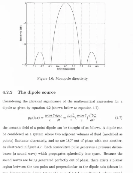
4.2.2 The dipole s o u rc e ...
51
4.3
Beamforming for a dipole s o u rc e ...
54
4.4 Source l o c a t i o n ...
58
4.4.1 Source o rien tation...
60
4.4.2 Source m e a s u re m e n t...
61
4.4.3 C onclusion...
61
4.5
Experimental v a l i d a t i o n ...
63
4.5.1 In tro d u c tio n ...
63
4.5.2 Experimental set-up ...
64
4.5.3 An acoustic s o u r c e ...
64
4.5.4 An aeroacoustic s o u r c e ...
68
4.5.5 Aeroacoustic testing ...
71
4.5.6 The search a lg o rith m ...
74
4.5.7 Source m e a s u re m e n t...
77
4.6
D isc u ssio n ...
79
5
M u ltip le sources
83
5.1 In tro d u c tio n ...
83
5.2 Twin sources ...
83
5.2.1
Dealing with m agnitude and p h a s e ...
90
5.2.2
Real and imaginary co m p o n en ts...
91
5.3 Calculating source strength ...
99
5.3.1
L im ita tio n s ...
103
6
G eneral d iscu ssion
104
6.1 Beamforming for specific a p p lic a tio n s...
104
6.2 Aeroacoustic s o u r c e s ...
106
6.3 Analysis te c h n iq u e s...
106
6.4 Summary of analysis t o o l s ...
107
6.5 General m e th o d o lo g y ...
108
6.6 D isc u ssio n ...
110
List o f Figures
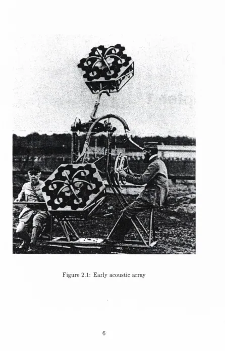
2.1
Early acoustic array ...
6
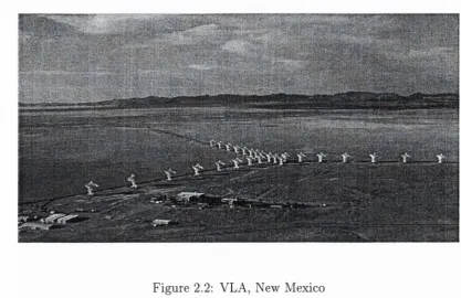
2.2
VLA, New Mexico ...
8
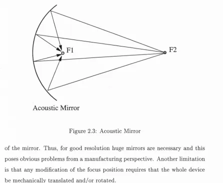
2.3
Acoustic M ir r o r ...
10
2.4
B e a m fo rm in g ...
12
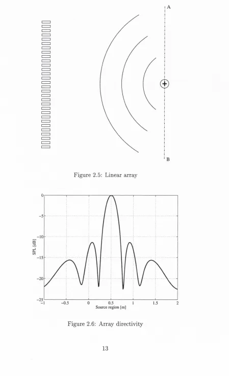
2.5
Linear a r r a y ...
13
2.6 Array directivity ...
13
2.7 Effect of source frequency ...
18
2.8 Effect of array l e n g t h ...
18
3.1
System reference f r a m e ...
21
3.2
Far-field s e t u p ...
23
3.3
Near and farfield directivities ...
27
3.4
Farfield directivity m an ip u latio n ...
28
3.5
Nearfield directivity m a n ip u la tio n ...
29
3.6
Apian model g e o m e tr y ...
31
3.7
Experimental s e t u p ...
32
3.8
Linear array setup and d ire c tiv ity ...
34
3.9
Cross array setup and directivity ...
35
3.10 Circular array setup and d ire c tiv ity ...
36
3.11 Array sensitivity for 6 0 0 H z...
38
3.12 Nearfield array sensitivity for 600H z...
39
3.13 Farfield array sensitivity for 600Hz ...
39
3.15 Modified nearfield array sensitivity for 600H z...
41
3.16 Modified farfield array sensitivity for 600Hz ...
41
4.1 The m o n o p o le ...
44
4.2 The d ip o le ...
45
4.3 The q u a d ru p o le ...
46
4.4 Sound pressure magnitudes on array for a monopole source . .
49
4.5 Monopole phase distributions before and after weighting . . .
50
4.6 Monopole d ir e c tiv ity ...
51
4.7 Sound pressure field of a d i p o l e ...
52
4.8 Polar Pressure Distribution of a D ip o le ...
53
4.9 Sound pressure magnitude distribution on array for dipole source 54
4.10 Fully reconstructed microphone signals for linear array . . . .
55
4.11 Dipole rotated through 3 0 ° ...
56
4.12 Array sound pressures for rotated d i p o l e ...
56
4.13 Beamforming with dipole s o u rc e ...
57
4.14 Microphone signals phase weighted for focus on dipole origin .
57
4.15 Microphone signals from one side of cancellation a x i s ...
58
4.16 Dipole o rie n ta tio n ...
60
4.17 Beamformer response before dipole modification - for a dipole
at 0.2m, o rie n ta tio n = 3 0 ° ...
62
4.18 Beamformer response after dipole modification for a dipole at
0.2, orientation=30°
...
62
4.19 Microphone a r r a y ...
65
4.20 Test s e t u p ...
66
4.21 Acoustic dipole directivity p a tte r n ...
67
4.22 M agnitude distribution for focus on s o u r c e ...
67
4.23 Phase distribution for focus on s o u rc e ...
68
4.26 Test setu p and resulting directivity p a t t e r n ...
72
4.27 M agnitude d istrib u tio n for aeroacoustic s o u r c e ...
73
4.28 Phase d istrib u tio n for aeroacoustic source
...
73
4.29 The dipole s i g n a t u r e ...
74
4.30 Phase d istrib u tio n as a function of focus position - aeroacoustic
d i p o l e ...
76
4.31 Phase distrib u tio n as a function of focus position - acoustic dipole 76
4.32 Phase d istrib u tio n as a function of focus position - acoustic
monopole ...
77
4.33 Beam form er m o d ifica tio n ...
78
4.34 Modified d ir e c tiv ity ...
79
4.35 Fourier transform from a single m icrophone
...
80
4.36 Fourier tran sfo rm after ordinary b e a m f o r m in g ...
80
4.37 Fourier transform after modified b e a m f o r m in g ...
81
5.1
Tw in source s y s te m ...
84
5.2
(a) 1.1m,
(b) 1 . 2 m ...85
5.3
(a) 1.3m, (6) 1 . 4 m ...
86
5.4
(a) 1.5m, (6) 1 . 6 m ...
87
5.5
(a) 1.7m,
(b) 1 . 8 m ...88
5.6
(a) 1.7m, (6) 1 . 8 m ...89
5.7
Real and im aginary distributions prior to f o c u s s i n g ...
91
5.8
Real and im aginary distributions for focus on point dipole . .
92
5.9
( a) 1.1m, (b) 1 . 2 m ...94
5.10 (a) 1.3m,
(b) 1 . 4 m ...95
5.11
( a) 1.5m, (b) 1 . 6 m ...96
5.12 (a) 1.7m,
(b) 1 . 8 m ...97
5.13
( a) 1.9m, (b) 2 m ...98
5.14 Complex distributio ns before and after fo c u ssin g ...
99
5.16 Real and imaginary distributions for varying source strengths .
101
C hapter 1
Introduction
1.1
E n gin eerin g and n oise
Noise pollution is an unfortunate consequence of many engineering develop
m ents and is one of the m ajor drawbacks of technological advance in automo
tive tran sp o rt systems. Although industrial noise has always been a problem,
recent legislation for environmental noise pollution has become more stringent
making the acoustic design of engineering systems a higher priority. Although
the full effect of noise on society is not yet fully understood, there is little
doubt th a t the psychological effects are very real. A comparison between a
m odern capital city and th at city two hundred years ago is most remarkable
for the difference in ambient noise. City sounds today are dominated by the
sound of automotive engine noise, whereas the ambiance of two hundred years
ago was dominated by the sounds of human conversation.
emphasises the necessity for improved research in the acoustic design of air
craft. In recent years the number of complaints received from residents living
near the m ajor European airports has increased substantially, despite large
reductions in noise levels, indicating th a t the public are becoming more sen
sitive to environmental noise and are less prepared to tolerate this intrusion
into their homes.
1.1.1
Aeroacoustic noise
The noise pollution evident around any modern airport is an example of aeroa
coustic noise, aeroacoustics being th a t branch of acoustics concerned with
sound generated by aerodynamic phenomena. Just as the mechanical work
ings of large industrial machinery generate noise, the aerodynamic ‘workings’
of modern aircraft also generate large amounts of unwanted sound. Aeroa
coustic systems tend to be more difficult to analyse than mechanical systems
however, due largely to the fact th a t the mechanisms responsible for the noise
are usually invisible and complex. While sound generated by mechanical sys
tems is due in the main to the vibration and contact of machine components,
sources of aeroacoustic sound are most often due to aerodynamic mechanisms
which remain undetectable to the naked eye, for example turbulence and fluid-
structure interactions.
The most obvious sources of aeroacoustic sound are manifest in the air
crafts’ propulsion systems, be they jet, propeller or otherwise. However, al
though a large proportion of the total sound energy can be attrib u ted to the
propulsion system, it does not account for all of the noise. As propulsion noise
is reduced, other less obvious sources of sound such as undercarriage noise or
flap-edge noise become more dominant.
Aeroacoustic sound is the result of disturbances in a sonic medium caused
aeroacoustic systems so difficult to analyse
1.1.2
R ed u cin g n oise levels
It is clear, th a t if the problem of environmental noise pollution is to be ad
dressed and successfully treated, sources generating noise and their associated
physical mechanisms m ust be evaluated and understood, as it is only then th at
b etter design techniques for the reduction of noise can be developed. The task
facing the acoustic engineer can be stated as follows: how can a noisy engineer
ing system be most thoroughly analysed, in order to identify the m ajor sources
of sound? The prim ary requirement is th a t the system be broken down into
its fundamental components, and th a t these components and their respective
interactions be studied to determ ine the mechanisms generating the resultant
acoustic field. Aeroacoustic systems generally consist of a large collection of
arbitrarily correlated individual source components. Thus, im portant sources
may often be embedded in a background of noise, making them extremely
difficult to identify. Separation of these components for examination necessi
tates a capacity for the exam ination of very specific regions of space-time, i.e.
regions of space over a given tim e period. This thesis is concerned with the
investigation and development of an experimental tool, based on the principles
of microphone array technology, capable of this kind of measurement.
1.2
T h e m icro p h o n e array
As sound is the direct result of physical mechanisms which cause distinctive
pressure disturbances in the surrounding medium, the resultant behaviour of
th a t medium gives valuable information concerning the nature of the source
mechanism. The microphone array is a device which can focus on specific
regions of space in order to determ ine the nature of the acoustic or aeroacoustic
sources in th at region.
aerody-namic phenomena. These generate distinctive acoustic fields depending on
the source mechanism, and so, through the medium of sound relay informa
tion which, when appropriately processed, can reveal the nature of the source.
The prim ary focus of this thesis is on two specific aspects of microphone array
applications.
• O p tim is a tio n The way in which the microphone signals are combined,
together with the characteristics of the system being analysed, play a
large part in determining the response characteristic which will result.
Through an examination of basic beamforming, and the m athem atical
formulation of this mechanism, the difficulty of antenna optim isation is
addressed.
Chapter 2
R eview o f array techniques
2.1
H istorical p erspective
Throughout the twentieth century advances in technology proceeded at what
appears to have been an exponential rate. Technologies which, at the begin
ning of the century were in their infancy, developed to become the foundation
technologies of today’s engineering environment. The concept of array pro
cessing is one such technology. Initially developed for m ilitary purposes, in
the form of radar and sonar, it has today become a vital element in areas such
as telecommunications and navigation.
Examples of array techniques can be found as early as the first world war
where arrays of acoustic receivers were used to ‘listen’ for the approach of en
emy aircraft, as shown in figure 2.1. This particular device could be manually
rotated so as to aim it in different directions, and thus identify the presence of
incoming aircraft. This technology was rapidly developed for m ilitary advan
tage in the form of radar and sonar detection systems. Radar, which was being
developed by the Germans as early as 1933, uses electromagnetic radiation to
search space for the presence of solid bodies. Portions of the electromagnetic
Figure 2.2: VLA, New Mexico
power in a given direction, thus avoiding radiation into redundant regions of
space. Much of the research in this area is concerned with the optimisation
of radiation patterns. Dolph [4] developed a technique which maximises ra
diation resolution, i.e. the m ajority of the signal power is concentrated in as
narrow a beam as possible. Bouwkamp et al. [5] argued th a t there is no exact
solution to the problem of optimum current distribution for linear radio anten
nae and they developed a method to realize any radiation pattern by suitable
choice of current distribution. Riblet, [6] extended the theory of Bouwkamp
to two-dimensional current distributions to enable the same radiation pattern
specification for planar antennae.
[image:22.545.69.487.28.298.2]ally applied to a collection of microphones (or hydrophones, depending on
the application), known collectively as an acoustic array. The layout of the
microphones depends on the system it has been designed to analyse. The mi
crophone signals can be processed individually and then combined in one of
any number of different ways (multiplied, added, convolved etc.), depending
on w hat is required of the measurement. The array treats incoming sound
waves in a similar fashion to the treatm ent of electromagnetic radiation by
radar systems, and, in the same way, is capable of discovering the direction
from which a given sound field emanates. Just as radar is used to determine
the positions of objects in space, an acoustic antenna can determine the source
of a given sound field.
Arrays can be used to analyse noisy engineering systems in order to obtain a
b etter understanding of the noise sources through more accurate measurement.
W ith this more fully developed understanding of the sources responsible for
the sound, the engineer is in a better position to reduce overall noise levels.
Meadows et al. [9] for example performed measurements on a NACA 632 — 215
wing section with a 30 percent chord half-span flap. Using two directional
arrays, correlated with an array of unsteady surface pressure transducers, they
identified th a t locally dom inant noise sources existed on the flap-side edge.
Before the most recent developments in computing power, acoustic mir
rors were the preferred tool of acousticians seeking to analyse complex noise
producing systems. The acoustic mirror is an acoustically reflective surface of
parabolic shape, with a microphone located at the inner focal point (shown in
figure 2.3 as F I). The m irror is arranged such th a t the area of interest lies at
the outer focal point (shown in figure 2.3 as F2). In this way the m ajority of
the system ’s energy is focused on the inner microphone, while sound generated
by regions away from the outer focal point is scattered so as to cause destruc
Acoustic Mirror
Figure 2.3: Acoustic Mirror
of the mirror. Thus, for good resolution huge mirrors are necessary and this
poses obvious problems from a m anufacturing perspective. Another lim itation
is th a t any modification of the focus position requires th at the whole device
be mechanically translated an d /o r rotated.
As long as digital signal acquisition and processing remained inefficient the
acoustic mirrors were a viable option. However, with the recent advances in
computing power, these devices have, for the most part, become redundant.
The speed at which d ata can be acquired and processed has given rise to a
renewed interest in microphone array systems. There has been an abundance
of research in the past few years in a wide variety of areas, from the tracking
of zooplankton [10] to jet noise source localisation [11].
2.2
B eam form ing and som e o f its problem s
[image:24.540.72.517.29.395.2]of using a number of transducers at discrete spatial locations in order to sam
ple a given wave field. The signals are then processed such th a t signal power
from a specified region is enhanced, whereas signal power from all other re
gions is attenuated. The underlying principle is quite simple; if a propagating
wave field is incident on a collection of transducers, it will arrive at each of the
transducers at a different time, depending on the source-transducer distance.
Because the relative time differences are simply dependent on the source po
sition, the transducer signals can be modified to eliminate the tim e difference,
or phase-difFerence in the frequency domain. The time differences are manip
ulated such th a t the tem poral coordinates of the microphone signals become
the same, thus forcing the signals into phase with one another with respect to
a specified source. In this way, those portions of the transducer signals which
came from a point in space defined by th a t set of phase shifts, when summed,
will interfere constructively. Similarly, portions of signals em anating from any
other region will interfere destructively. By appropriate manipulation of the
signals’ phases the focus of the array can be shifted about in space, boosting
the signal to noise ratio of specified regions. This technique can be thought
of as an adaptable acoustic mirror. Whereas variation of a m irror’s focus
position and resolution requires mechanical alteration of the device, all array
adaptation can be achieved electronically. Figure 2.4 illustrates this technique.
2.2.1
D irectivity
DELAY 4 DELAY 1
DELAY 2
DELAY 3
Figure 2.4: Beamforming
SP
L
[dB]
Figure 2.5: Linear array
-1 0
-1 5
-20
-2 5
-0.5 0.5
Source region [m]
[image:27.540.74.523.33.769.2]the measurements which can be taken, for example Marcolini and Brooks [8]
developed a technique which produced constant measurement resolution for
different frequencies and applied it to a helicopter rotor in order to obtain
quantitative measurements.
2.2.2
Source localisation in acoustics and aeroacoustics
m ultiplicative signal processing and additive processing. They found th a t by
using m ultiplicative m ethods th e resolution of an a rra y ’s response could be
improved. A gain th is technique was for the case of very high SNR.
T he spatial resolution of an array is a function of th e frequency of th e source
being m easured, which m eans th a t th e characteristics of a given m easurem ent
depend on th e frequency of interest. M arcolini and Brooks [8] addressed this
problem using a m eth o d which can be illu strated more clearly thro u g h an ex
am ination of figure 2.6. They considered th eir
effective
m easurem ent region to
be th a t region bounded by th e -3dB points, although in th eir case the m easure
m ent region was two dim ensional, and so th e -3dB points are represented by a
contour line. T he size of this region (i.e. th e resolution of th e array) depends
on th e source frequency, clearly an undesirable effect. M arcolini and Brooks [8]
developed a blending type procedure in order to generate constant beam -w idth
for varying source frequency. In effect this m eant th a t regardless of th e source
frequency, th e position of th e -3dB points rem ained constant, giving a con
s ta n t effective m easurem ent region. The array system which they developed
was for th e analysis of helicopter rotor noise. They successfully achieved spa
tial resolution of th e m ain directional lobe which was independent, not only
of frequency, b u t also of look angle. They obtained good agreem ent in a com
parison of th e sp ectral results from the array w ith predicitons of broad b and
self noise, and w ith to ta l ro to r noise m easurem ents obtained from individual
microphones of th e array. Due to the anechoic environm ent, side-lobe position
and size was no t a m ajo r concern.
included th e blending procedure of M arcolini and Brooks. This application
was for high frequency source analysis (2 — 30kHz ) .
At these fequencies there
will be a large num ber of sidelobes very close to the m ain lobe and so it is vital
th a t th e gain of the array is optim ised, in order to minimise contam ination.
For low fequency applications this optim um gain is not as im p o rtan t because
the first sidelobe will often lie outside th e sound generating region. T his will
be dem onstrated in the case stu d y discussed in chapter 3.
2.2.3
M icrowave an ten n ae
As th e beam form ing principle derives from antenna theory it is useful to ex
am ine some of the work conducted in this area. Radio antennae use th e sam e
principle in order to achieve directional electrom agnetic radiation. M uch of
the radio literatu re is concerned w ith the synthesis of optim um directivity
p atte rn s for linear point arrays, or antenn ae w ith continuous current d istrib u
tions. Schelkunoff [16] form ulated th e problem according to a far-field model,
and using th is model approxim ated th e directivity of an array as a polyno
mial. Dolph [4] was concerned w ith th e control of m ainlobe w idth and sidelobe
suppression, and he developed a technique which was extended by R iblet [6]
to two dimensions. D uham el [17] m odified the techniques of Dolph and Ri
blet so th a t a common design procedure could be used. Ziehm [18] worked
on th e optim isation of circular array directivity while Elliot et al. [19] were
concerned w ith planar system s. W oodw ard et al. [20] present a m ath em atical
theory for two-dim ensional arrays which suggests the possibility of unlim ited
directivity control, although in practice th e application of this theory is lim
ited by unrealistic excitation am plitudes. T he work of Dolph and R iblet was
adapted for application to an acoustic an ten n a by P ritch ard [21], who realised
the p o ten tial of these techniques for application to acoustic arrays.
was specified the minor lobe levels could be minimised. Further to these ob
servations, Dolph [4] showed th a t the relevant element excitations required to
produce an equal minor-lobe pattern could be found. The m ethod involved
transform ing the array’s directional characteristic to a polynomial in a suitable
variable, and then applying an appropriate transform ation with Tchebycheff
polynomials - which possess the property th a t all extrem a are of the same am
plitude. Pritchard [21] extended these techniques to steered or ‘com pensated’
arrays. The importance of transducer spacing was discussed at some length
and it was noted, in particular, th a t spacings equal to the sound wavelength
resulted in unacceptably large secondary lobes. Arrays with spacing equal to
or less than a wavelength are referred to as ‘super-gain’ arrays by Riblet [6].
In present day array design, it is a prerequisite th a t the transducer spacing
be less than half a wavelength. Pritchard [21] also found th a t as the array
length was increased the m ajor lobe width decreased (for constant transducer
spacing), a now well established consequence.
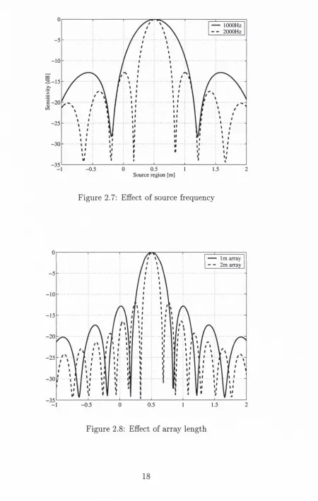
The effect of source frequency and array length on the response of an array
are illustrated in figures 2.7 and 2.8. For a system set-up as in figure 2.5,
w ith the source region at a distance of
2m
from the array, and for a thirty
element,
2m
array, the directivities for monochromatic sources of
lOOOHz
and
2000Hz
are shown in figure 2.7. It can be seen clearly th at as the source
frequency is increased the array’s resolution improves. The effect of array
length is illustrated in figure 2.8 which shows directivities for 1 and
2m
arrays
in the presence of a
2000Hz
source.
2.3
S um m ary
lOOOHz 2000Hz
- 1 0
1 - 2 0
-25
-3 0
-35
0.5 Source region [m]
-0.5 1.5
Figure 2.7: Effect o f source frequency
Im array 2m array
-5
- 1 0
-1 5
-2 0
-2 5
-3 0
-35
0.5
-0.5 1.5
[image:32.540.73.523.44.754.2]array be designed so as to minimise the potential for spurious interpretation
and contamination from unwanted sources. This requires th a t the array re
sponse characteristics be well known for all system set-ups. Emphasis is placed
on the necessity for directivity control, or where this is not possible, the need
for a thorough knowledge of the response characteristics of the array.
There are two specific aspects of array measurement which will be investi
gated in this work. The first is the problem of directivity control, an area which
has received much attention in the area of microwave antenna, but which has
not been fully exploited in acoustic and aeroacoustic applications. The second
aspect is the identification of specific types of aeroacoustic source. If an array
is to be used to its full potential, it is crucial th at both these aspects be given
C hapter 3
D irectiv ity m odelling and
control
3.1
Introduction
The dependence of array response on param eters such as source frequency,
array geometry, position and orientation poses real problems in the practi
cal implementation of these devices. The external control of directivity is
something which has been dealt with in some detail in telecommunications
research, as was seen in the last chapter. Similar control has not been used as
extensively however in acoustic array design, and so, in this chapter the prob
lem of acoustic antenna optim isation is addressed. The problem is formulated
m athem atically according to both near and far field models, thus allowing the
specific difficulties of directivity control to be identified.
3.2
N ear field form ulation o f array response
Using the coordinate system shown in figure 3.1, for a microphone at point M,
S (xs,ys,zs)
Rf
y
M (xm,ym,zm)
F (xf,yf,zf)
Figure 3.1: System reference frame
source is given by
p - j k R p
= ^
(3.1)
Equation 3.1 is the monochromatic solution of the acoustic wave equation.
When this signal is weighted for focus on point F it becomes
„ j k ( R f - R p )
P{k, Rp,
R f )=
(3.2)
Which in terms of the cartesian coordinates of the source, microphone and
focus position is
P { k , R , ) =
A'K[{Xm -
XsY +
{Vm ~ VsY
+
(^m “
(3.3)
This equation represents a single phase-weighted microphone signal, thus the
array output can be w ritten as
4ir
l ( l m- x,Y
+
( t / „-
y,Y
+ (z„ -
2 , ) ’ ] ' / ^(3.4)
q _ y NEquation 3.4 is the array response to a sound source at position S, when
the focus position is F, for microphone coordinates
{xm,ym, ^m)
and
m
=
1 :
N ,
where
N
is the total number of microphones. This represents the
sensitivity of the array at spatial coordinate
{xf,
y/,
zj )
and constitutes a single
equation with
3 N
unknowns, or
4 N
if microphone weights are included. This
is clearly insoluble. However, given th a t a selection of spatial coordinates
and their corresponding requisite sensitivities can be specified, this equation
can be extended to a system of 4iV equations with the same 4A^ unknowns
(microphone coordinates and weights). The equation system can be easily
over determined by increasing the number of spatial coordinates accordingly.
It would seem from this th a t any arbitrary directivity pattern can be spec
ified and a set of microphone coordinates an d /o r coefficients calculated, in
order to achieve th a t directivity. Unfortunately, due to the ill-conditioned
nature of this equation system, obtaining a useful solution is virtually im
possible. This ill-conditioning is due to a long established tenet of acoustics,
namely -
for any given wave field, there exists no unique solution representing
the source.
If the array elements are thought of as a collection of point sources,
and the directivity p attern the resultant sound field (which is m athem atically
identical to the more usual formulation), then it becomes clear th a t any exact
directivity control will not be achieved by straightforward means. It may be
possible, using very powerful computers, to design optimisation algorithms ca
pable of perfect directivity control, however in the absence of supercom puting
it is neccessary to consider an alternative approach. One such approach is
to formulate the problem for a farfield setup, and examine how the govern
ing equations change. This is addressed in the next section using the radio
3.3
Far field form u lation o f array resp on se
W hen considering an array system located in the far field of an acoustic source,
th e problem is exactly analagous to a radio tra n sm ittin g antenna. T his is
because th e targ et region of a radio tra n s m itte r lies in the em m iter’s far field,
so th a t th e wave field in th a t region can be considered to consist of plane
waves. It is for this reason th a t the far field assum ption is valid for all radio
tran sm itters. Much of th e successful directivity control reported in the radio
lite ra tu re is based on th e foundation work of SchelkunofF [16], which expresses
th e problem in concise m athem atical term s.
Consider th e system shown in figure 3.2, consisting of a linear array of
receivers, equally spaced and in th e far field of some acoustic source, whose
wave field approaches a t velocity c (or wavenumber
k
=
2'Kflc).
Because th e
receivers are in the farfield, the waves can be considered plane when they arrive
a t the array. T he signal received on any of the transducers can be w ritten as
d
P = A n C o s { n k d C os6) (3.5)
where d is defined in figure 3.2. The nkdCosO term here accounts for the
phase-shift due to the signal arriving at each transducer at a different tim e.
W riting th is in th e more general form of
P = AnZ (3.6)
where
z = (3.7)
and
4> = kdCosO — l3 (3-8)
where is the phase m odification associated w ith focussing, the array output
can now be w ritten as
P = \Aq + A \Z + A ^ ^ + Asz^ + ... + Aji—iz^ ^ + AnZ^\ (3-9)
It can be seen then th at when the array response is formulated according to
the far field assum ption, it can be w ritten as a polynom ial. T his leads to
Schelkunoff’s first theorem , which states that every linear array with com
mensurable separations between elements can be represented by a polynom ial
and every polynom ial can be interpreted as a linear array. It can be seen from
equation 3.8 th at 0 is a function o f 6, i.e. the angle between the array and
any look direction. 0 is a real valued function, so th at the absolute value o f z
is equal to 1, im plying th a t 2 always lies on the circumference of a unit circle.
If the spacing between the elem ents is equal to A /2 (where A is the sound
wavelength) then the range of z is equal to 27t, and as the look direction,
changes from 0° to 180°, z describes one com plete circle. In this case there is a
\ I 2 , z
describes a sem i-circum ference. So, depending on th e elem ent spacing
and th e source frequency, regions of space correspond to different regions of
th e circumference of th e u n it circle.
C onsideration of th e fact th a t th e pro d u ct of two polynom ials is a poly
nom ial leads to Schelkunoff’s second theorem , which states th a t
there exists
a linear array with a directivity (or space factor) equal to the product o f the
directivities o f any two linear arrays.
An example can illu strate th is point.
Consider th e two elem ent array whose directivity is given by
Pi = \l + z\
(3.10)
m ultiplying this directivity by itself gives
P2 = |1 + 2|2 = 11 + 22 + 2^1
(3.11)
which is a three elem ent array w ith transdu cer m agnitudes of 1,2 and 1. From
theorem 2 it can be said th a t in a direction where Pi has a sensitivity of
P
2will have a sensitivity of |.T h is shows th a t th e microphone signals of an array
can be weighted such as to modify th e directivity p a tte rn , and th e relationships
between these weight d istrib u tio n s and the resulting directivities can be known
through th e knowledge of th e directivity p a tte rn of th e equivalent array to
which these weights correspond.
Nov/ consider a pair of tran sd ucer signals of am plitude 1,
—t
P = \ z - t \
(3.12)
The complex num ber
z — t
represents a line from
2to
t,
so th e sensitivity of
the two elem ent system in th e direcion
2: is given by th e length of the line
zt.
For the sensitivity to be zero in any direction, the null of the polynom ial
\z — t\
m ust be in the range of z and m ust be on th e circumference of th e u n it circle.
Now, any polynom ial of degree (n —1) has (n —1) roots and can be factorised
into (n — 1) binom ials, thus the sensitivity given in equation 3.9 can be w ritten
as
Each of these binomials represents the directivity of a two element array, which
leads to Schelkunoff’s third theorem which states th a t
the directivity of a linear
array of n elements is the product of the directivities o /(n —1)
virtual couplets,
with their null points at the zeros of P.
The implication of Schelkunoff’s work for acoustic receiving arrays is th a t
the positions of the nulls of an array’s directivity pattern can be chosen by
generating a polynomial whose roots lie at the appropriate positions on the
unit circle. The coefficients of this polynomial are then the weights which need
to be applied to the elements of the array system in order to achieve the said
null positions.
3.4
A p plication o f SchelkunofF’s theory
The applicability of Schelkunoff’s theory to an acoustic array for both near
and farfield formulations was examined using M atlab based models. Directiv
ity patterns were generated in order to compare true array directivity (nearfield
formulation) with the approximated directivity (Schelkunoff’s farfield polyno
mial formulation), and, using these, the effect of sidelobe null specification on
the nearfield model was assessed.
3.4.1
D irectiv ity com parison
Near and far-field directivity patterns were generated through numerical imle-
mentation of equations 3.9 and 3.4 . These are shown in figure 3.3 for a source
frequency of
I k Hz .
The discrepancy between the models is due to the approximate nature of
the farfield formulation. Schelkunoff represents the array sensitivity using a
polynomial, whereas this is not actually the case. The true m athem atical for
Schelkunoff model — Nearfield model
- 1 0
-20
;i;r-30
-50
-60
-70
80 100
Look direction [deg]
120 140 160 180
Figure 3.3: Near and farfield directivities
able, at least qualitatively, in the nearfield
Ccise.The following example was
used to investigate this possibility. Consider a
3m
linear array with thirty
commensurably spaced elements taking measurements from a linear source
region, parallel to the array axis, and at a distance of 7m. The directivity
for this sytem, according to Schelkunoff’s model is shown in figure 3.4. The
sidelobe nulls directly adjacent to the mainlobe are located at 78° and 102°.
Using the method described in the previous section the directivity can be
manipulated in order to shift these nulls, and this can be done exactly. In
this example, a decision is taken to move the nulls to 80° and 100°. Using
these positions a polynomial is generated whose roots lie at these positions
and the coefficients of this polynomial are the weights necessary to produce
the desired effect. It is shown in figure 3.4 th at the nulls are shifted to the
locations specified. A side effect of this directivity manipulation is a reduction
in mainlobe level and an increase in sidelobe levels. If the nulls are moved
in the other direction, the side effects are reversed, i.e. the mainlobe level is
-1 0
-20
-30
-5 0
O riginal directivity - - M odified directivity
-70
100 110 120
Look direction [deg]
Figure 3.4: Farfield directivity m anipulation
of benefit for an actual acoustic array, the effect on the nearfield model must
be assessed, so, using the same test param eters the procedure was repeated
using the nearfield formulation. Figure 3.5 shows the result.
It is clear th a t the same effect has been produced on the nearfield model.
The sidelobes adjacent to the mainlobe have been shifted by approximately
the same amount as was achieved using the farfield formulation, and a similar
change is evident in both mainlobe and sidelobe levels. From this it is clear
th at the technique can be used effectively with a real array. Depending on
the modification required, these numerical models can be used to identify an
appropriate set of microphone weights.
3.5
A case stu d y
To illustrate the need for optimising both array geometry and processing for
O riginal directivity - - M odified directivity
- 1 0
-15
m - 2 0
-30
-35
-4 0
-45
100 110 120
L ook direction [deg]
Figure 3.5: Nearfield directivity manipulation
APIAN (Advanced Propulsion Integration Aerodynamics and Noise). The
objective of this project is to study the aeroacoustics of installed high-speed
propellers. A microphone array is to be used in these tests to identify the
contribution to the overall sound field of a single propeller. This requires th at
contam ination from the second propeller, as well as acoustic reflection from
the fuselage, be minimised. Thus, as the m ajor source of contam ination in this
case is the second propeller, the prim ary design criterion for the array is th a t
the contribution of this propellers be entirely filtered out. It is not often the
case in array applications where there are two such coherent sources of noise
of similar orders of m agnitude and frequency, and so, it is often sufficient
to design an array with good gain characteristics and then not worry about
sidelobe contamination. In this case however, as the source of contam ination
is at exactly the same frequency, and of similar strength, it is necessary to
achieve a higher degree of attenuation. This can be achieved by ensuring th at
the second propeller lies in a region of the sensitivity pattern where attenuation
were developed for this application based on test param eters such as model
size, source frequency, array-source distance, and the relative strengths and
weaknesses of each was assessed in order to choose the most suitable design.
3.5.1
T est set-up
The APIAN model geometry is shown in figures 3.6(a) and
(b).
The model
has a wingspan of 3m and the propeller nacelles are separated by a distance
of Im . This means th a t at the fundam ental frequency, the array sensitivity
pattern must be such th a t the distance between the mainlobe peak and the first
sidelobe trough is roughly equal to Im . The propellers, which have a diam eter
of 0
.5
t t i,are not shown in this diagram. The model is to be tested in the closed-
loop open-section wind tunnel at DNW (the Dutch-German wind tunnel), and
will be positioned as shown in figure 3.7. The DNW open-section facility
has anechoic treatm ent which eliminates acoustic reflection. This means th at
sidelobes pointing away from the source region are of no concern. In view of
this the directivity pattern of the array only needs to be considered in the
region of the aircraft model. The model is approximately 5m from the wind
tunnel nozzle and at a height of 3m. Acoustic measurements will be taken
using an out-of-flow microphone array positioned immediately below the wind
tunnel nozzle. At this point the array is a close as possible, in term s of angle, to
the propeller axis and will give a measure of the sound radiated in the forward
direction. This position gives a source-array distance of approximately 7m. If
this distance is known, and the positions of the main sources of noise are known
(i.e. the propellers) an array geometry can be chosen with an aperture such
th a t one of the propellers lies in the trough of a sidelobe for the frequency
of interest. For these particular tests the rotational speed of the propellers
is
SOOOrpm,
which for a six bladed propeller corresponds to a fundam ental
-0.5
-2
-2.5
- 3
-1.5
0.5 0 -0.5 ■1
1.5 1
1 0-2
8 O'
a 0
3 - 0 -I 1.5
D istance [m]
(a)
( b )
0 .5 0 - 0 .5 - 1 - 1 .5
D istance [m]
3 -1
E 0
-5 - H ; :
- 2 - i
- 3 - ;
-4
-W ind tu nnel nozzle
APIAN m odel
1---1--- r 2 1 0 Distance [m]
~ r
-2 - 3
“ T - 4
(a) Elevation
i APIAN rtlodel 5
i
I
\
i 5 ;
: \
1
Wind tunr el n o zzle
____ 1 ... 1 , , 1.,
2 I I I_________I I I I I_________ I I________I 6 5 4 3 2 1 0 -1 - 2 - 3 - 4
Distance [m]
{b) Plan
3.5.2
T h e linear array
A linear microphone array gives good spatial discrimination along an axis
parallel to its own axis, in other words, it can not spatially filter along axes
perpendicular to its own. Thus for a horizontal linear array the sensitivity
pattern is a function of horizontal distance only. As the source distribution
in the APIAN case is approximately linear, a linear array is an appropriate
design. The setup showing a linear array is shown in figure 3.8(a). For a
fundamental frequency of 800//^ the optimum array length is 3m. At this
length, the right hand propeller lies in a region of the sensitivity pattern where
the attenuation is of the order of
—28dB.
This is shown in figure 3.8(i).
3.5.3
T he cross array
The second array design considered for these experiments was a cross array,
which gives better discrimination for a planar source region. An optimum cross
array for the APIAN setup is one with a length of
Am
(this is the distance from
the tip of one arm to the tip of its opposite member). This setup is shown in
figure 3.9(a). It can be seen th a t the array is physically very large, in fact it is
obstructed by the wind tunnel nozzle. The sensitivity pattern for this array is
shown in figure 3.9(6). Good attenuation is again achieved on the right hand
propeller, and a certain amount of vertical discrimination also results. This is
manifest in the improved attenuation seen in certain regions of the fuselage.
This design gives a b etter sensitivity pattern in terms of better attenuation
on the model fuselage, but the size of the array poses a problem.
3.5.4
T he circular array
Another possible geometry is the circular array, and it is found th at for this
case the optimum geometry consists of a 2.5m diam eter circular arrangement,
shown in figure 3.10(a). The sensitivity pattern for this array is shown in fig
-a
x
is
[m
]
Wind tunnel nozzle
2
-APIAN mode)
0 --1
--3 Linear array
x -a x is [m] - 4
y -a x is [m]
(a)
8
:
1.5
---7
-1 0.5 07----0.5-7- -1 - 1.5 -3
SensFtfvily [dB]
(b)
Sersiifvity (00)
i b )
T
J
T
S e n s itiv ity [dB]
hand propeller. As was the case with the cross array, this array geometry
provides a degree of vertical discrimination, again showing better attenuation
on regions of the fuselage than can be achieved with a linear array. However,
as was the case with the cross array, it is physically too large.
3.6
D iscussion
The previous section illustrated the performance potential of a number of
different array geometries. The purpose of this discussion is to illustrate the
process whereby an optimum array can be chosen based on its performance
characteristics with respect to a specific system.
It can be seen in each case th a t an optimum array size can be chosen so
as to ensure th a t the right hand propeller lies in a region of high attenuation.
However, a difficulty with these planar designs becomes clear as focussing is
attem pted at frequencies other than the fundamental. In these cases the side-
lobes will move, causing the amount of attenuation at the right hand propeller
to change. This means th a t measurement at frequencies other than the fun
dam ental will be prone to varying degrees of contamination. In the case of the
linear array however, through application of the technique described earlier in
this chapter the sensitivity pattern can be m anipulated so as to ensure th a t
the propeller remains in a region of high attenuation. This is illustrated by
changing the measurement frequency to 600ii/z and observing the change in
array sensitivity. The result is shown in figure 3.11. It is clear from this th a t
the beamformer is no longer performing at its optimum. The attenuation on
the second propeller has now changed from
—2SdB
to
—9dB.
This will result
in considerable contamination of the measurement. Another consequence of
this change in array sensitivity is th a t measurements taken at the two different
frequencies will not be comparable, due to the varying degrees of contam ina
0
- 8
-10
- i :
- u
-16
- I S
-20
F ig u re 3.11: . \ r r a y s e n s i t iv i ty for 600Hz
th e s e cond p ro p e lle r has now c h a n g e d from —2 S d B to —9 d B . T h i s will r e s u lt
in c o n s id e r a b le c o n t a m i n a t i o n of th e m e a s u r e m e n t. .A.nother c o n s eq u e n c e of
th is c h a n g e in a r r a y s e n s itiv ity is t h a t m e a s u r e m e n t s ta k e n a t th e two different
frequencies will n o t be c o m p a r a b l e , d u e to th e v a ry in g degrees of c o n t a m i n a
tion. U sing th e null s p e cific a tio n te c h n iq u e b a s e d on S c h e lk u n o ff’s t h e o r y of
a rr a y s , th e s e n s itiv ity p a t t e r n c a n be m a n i p u l a t e d in o r d e r to r e - o p tim is e the
a r r a y s y s te m . A sim plified r e p r e s e n t a t i o n of t h e d ire c tiv ity p a t t e r n is show n
in figure 3.12. For th e s y s te m s e t u p th e p r o p e lle r b e in g m e a s u r e d is lo c a te d
a t 90° a n d th e second p ro p e lle r a t 98°, i n d i c a t e d by th e d a s h e d line. From
figure 3.12 th e m a x i m u m a t t e n u a t i o n is sh o w n a t 101°, so a m o d ific a tio n of
3° is req u ire d in o r d e r to re -o p tim is e th e array. T h e d i r e c tiv ity as r e p r e s e n te d
by SchelkunofF’s a p p r o x i m a t i o n is sh o w n in figure 3.13. B ecause o f th e dis
c re p a n c y b e tw e e n th e two f o r m u la t io n s it is n o t possible to give th e a c tu a l
lo c a tio n of th e second p r o p e lle r for null spe cific a tion. However, th e a m o u n t
of m o d ific a tio n re q u ir e d is know n, a n d so an a p p r o p r i a t e null lo ca tio n c an be
-10
-15
a -20
> -2 5
-35
-40
-45
-50
100 105 110 115
Look direction [deg]
Figure 3.12: Nearfield array sensitivity for 600Hz
0
- 1 0
-2 0
-3 0
-4 0
-5 0
-6 0
100 105 110 115
65 70 75 80 85 90 95