The Unified Transform for a Class of
Reaction-Diffusion Problems with Discontinuous
Time Dependent Parameters
M. Asvestas, E.P. Papadopoulou, A.G. Sifalakis and Y.G. Saridakis
Abstract—Reaction-diffusion mathematical models for study-ing, among others, highly diffusive brain tumors, that also take into account the heterogeneity of the brain tissue, are frequently used in recent years. Current work, considers a generalized class of such reaction-diffusion models that also allows both diffusion and reaction parameters to depend continuously in time. A series of transforms are applied to produce an integral representation of the problem’s solution. Main approach used is Fokas unified transform which yields novel integral representations of the solution in the complex plane that, for appropriately chosen integration contours, decay exponentially fast and converge uniformly at the boundaries. Combining these method-inherent advantages with numerical integration techniques on hyperbolic contours, we produce an efficient method, with fast decaying error properties, for the solution of the multi-domain reaction-diffusion model problem.
Index Terms—Reaction-Diffusion PDEs, Brain tumors, Uni-fied transform, Fokas method.
I. INTRODUCTION
Reaction-diffusion linear PDEs have been the core biomathematical model for studying highly invasive and aggressive forms of brain tumors for many years now (e.g. [10], [7] and the references therein). The driving differential equation of the basic model has the form
∂¯c
∂¯t =∇ ·( ¯D∇¯c) + ¯ρc,¯ (1) where¯c(¯x,¯t)denotes the tumor cell density at locationx¯and time¯t,ρ¯denotes the net proliferation rate (0.012 1/day, cf. [2]), andD¯ is the diffusion coefficient representing the active motility of malignant cells (0.0013cm2/day, cf. [16]). The model also considers zero flux boundary conditions, which impose no migration of cells beyond the brain boundaries, and an initial condition ¯c(¯x,0) = ¯f(¯x), where f¯(¯x) is the initial spatial distribution of malignant cells.
Predicting a linear growth of the mean tumor diameter on MRI, Swanson (cf. [14], [15]) incorporated brain’s tissue heterogeneity (white-gray matter) into the basic model by consideringD¯ be defined by
¯
D≡D¯(¯x) =
( ¯
Dw, x¯ in white matter(¯x∈Ωw)¯ ¯
Dg, x¯ in gray matter(¯x∈Ω¯g)
, (2)
Manuscript received March 10, 2015; revised April 10, 2015.
This work was supported by the ESF and Greek national funds through the operational programEducation and Lifelong Learningof the National Strategic Reference Framework (NSRF) THALES (Grant number: MIS-379416).
All authors are with the Applied Math & Computers Lab, Technical University of Crete, 73100 Chania, Crete, Greece
Email of the corresponding author : [email protected]
whereD¯w andD¯g are scalars withD¯w>D¯g.
The above important model problem may be considered as part of a more general class of problems characterized by the fact that both diffusion and reaction parameters depend also in time. To be more specific, we’ll assume that
¯
D(¯x,t¯) = ¯χ(¯t) ¯D(¯x) and ρ¯≡ρ¯(¯t), (3)
where χ¯(¯t) 6= 0 and ρ¯(¯t) 6= 0 are continuous functions of
¯
t. In such a case, models that would, for example, allow both motility and proliferation of malignant cells to change in time are also included.
Assuming, for compatibility purposes, the same physical units and using the dimensionless variables (see also [14], [15] for an analogous treatment)
t= ¯ρ0¯t , x= r ρ¯
0
¯
χ0D¯w ¯
x , χ(t) = χ¯( ¯ρ0t¯) ¯
χ0
, γ= ¯
Dg ¯
Dw
,
(4) hence
D≡D(x) =
(
1, x∈Ωw
γ, x∈Ωg , D(x, t) =χ(t)D(x), (5)
ρ≡ρ(t) = 1 ¯
ρ0
¯
ρ( ¯ρ0¯t), f(x) = ¯f r ρ¯
0
¯
χ0D¯w ¯
x
, (6)
and
c(x, t) = χ¯0 ¯
Dw ¯
ρ0N0
¯
c
r ρ¯ 0
¯
χ0D¯w ¯
x,ρ¯0¯t
, (7)
withN0= R ¯
f(¯x)dx¯ to denote the initial number of tumor cells in the brain at¯t0= 0,ρ¯0= ¯ρ(¯t0)andχ¯0= ¯χ(¯t0), one may easily arrive at the dimensionless equation
∂
∂tc(x, t) =∇ ·(D(x, t)∇c(x, t)) +ρ(t)c(x, t). (8) Referring, now, to the above equation we proceed in the next sections as follows:
• Initially, by using appropriate transformations and
change of variables, we reduce the above equation into an equivalent one with constant diffusion coefficient.
• In the sequel, for the one space dimension problem and by using the Fokas unified transform method (cf. [3], [4]), we produce an integral representation of the solution in the complex plane that, for an appropriately chosen integration contour, decay exponentially fast.
• Finally, we apply efficient numerical integration tech-niques, with fast decaying error properties, for the numerical evaluation of the solution’s integral represen-tation.
II. INTEGRALREPRESENTATION OF THESOLUTION
A. Equivalence Transformations
Let us first show that:
Lemma 1. If c(x, t) satisfies equation (8) and u(x, t) is defined by
u(x, t) =e−R(t)c(x, t) with R(t) =
Z t 0
ρ(s)ds , (9)
thenu(x, t)satisfies the equation
∂
∂tu(x, t) =∇ ·(D(x, t)∇u(x, t)) . (10)
Proof: Observing that R˙(t) = ρ(t) and differentiating (9) with respect oft, it can be easily shown that
e−R(t)∂
∂tc(x, t) = ∂
∂tu(x, t) +ρ(t)u(x, t). (11) Multiplication now of equation (8) by the factore−R(t)yields
e−R(t)∂
∂tc(x, t) =∇·(D(x, t)∇u(x, t))+ρ(t)u(x, t), (12) which combined with relation (11) completes the proof.
Recalling, now, the form ofD(x, t)form (5), we can easily show that:
Lemma 2. If u(x, t)satisfies Lemma 1 and
τ≡τ(t) =
Z t 0
χ(s)ds , (13)
thenu(x, τ)satisfies the equation
∂
∂τu(x, τ) =∇ ·(D(x)∇u(x, τ)) . (14)
Proof: Upon writing D(x, t) = χ(t)D(x) equation (10) of Lemma 1 becomes
∂
∂tu(x, t) =χ(t)∇ ·(D(x)∇u(x, t)) . (15) Apparently, now, the fact that
∂
∂tu(x, t) = dτ dt
∂
∂τu(x, τ) =χ(t) ∂
∂τu(x, τ), (16) completes the proof.
B. The unified transform for the1 + 1 problem
In view of Lemmas 1 and 2, the dimensionless IBVP problem in 1+1 dimensions may be written as
uτ = (Dux)x, x∈[a, b], τ >0
ux(a, τ) = 0 and ux(b, τ) = 0
u(x,0) =f(x) := M
P
i=1
δ(x−ξi), ξi∈(a, b)
, (17)
whereD andτ are as defined in (5) and (13), respectively, andδ(x)denotes the Dirac delta function.
Due to brain tissue heterogeneity, the domain [a, b] is considered partitioned inton+ 1regionsRj := (wj−1, wj), witha≡w0 < w1 < w2< . . . < wn < wn+1 ≡b, and if, for somej,Rj is white matter region, then Rj−1 andRj+1 are grey matter regions. Thus, forx∈Rj, j= 1, . . . , n+1,
we denote the dimensionless diffusion coefficientD(x)as
D(x) =γj=
(
1, when Rj ⊆Ωw
γ, when Rj ⊆Ωg
. (18)
Furthermore, notice that the parabolic nature of the problem directly implies continuity of bothu and Dux across each
interface pointwj. Hence, for eachj= 1,2, . . . , nwe have
u(wj, τ) := lim x→w+j
u(x, τ) = lim x→w−j
u(x, τ) (19)
Dux(wj, τ) := lim x→w+j
D(x)ux(x, τ) = lim x→w−j
D(x)ux(x, τ).
(20) Let, now,u(j)(x, τ)denote the solution of the multi-domain problem defined over Rj := {wj−1} ∪ Rj ∪ {wj} = [wj−1, wj]. Namely, for j= 1, . . . , n+ 1,
u(j)(x, τ) :=
u(x, τ), x∈Rj
limx→w+
j−1u(x, τ), x=wj−1
limx→w−
j u(x, τ), x=wj
, (21)
and, naturally,
u(xj)(wj−1, τ) := limx→wj−1+ ux(x, τ)
u(xj)(wj, τ) := limx→w−
j ux(x, τ)
. (22)
Apparently then,
u(τj)= (γjux(j))x=γju(xxj) , (23)
while, recalling the constrains (19)-(20), there also holds: (
u(j)(w
j, τ) = u(j+1)(wj, τ)
γju
(j)
x (wj, τ) = γj+1u (j+1)
x (wj, τ)
. (24)
Observe, now, that the formal adjoint u˜(j) satisfies the equation
−˜u(τj)=γju˜(xxj) . (25)
Then, by multiplying equations (23) and (25) by u˜(j) and u(j), respectively, and subtracting the resulting equations, we obtain that
(u(j)u˜(j))τ−(γju(xj)˜u
(j)−γ
ju(j)u˜(xj))x= 0. (26)
Taking, also, into consideration that a one-parameter family of solutions of (25) is given by
˜
u(j)(x, τ;k) =e−ikx+γjk2τ, k∈
C (27)
equation (26) becomes
(e−ikx+γjk2τu(j))τ−(e−ikx+γjk2τγj(u(j)
x +iku
(j)
))x= 0
(28) which is the divergence form of equation (23). Integrating, now, over the region Aj :={(x, τ) :x∈Rj, 0≤τ ≤T}
and using Green’s Theorem we obtain that:
wj
Z
wj−1
e−ikxf(j)(x)dx− wj
Z
wj−1
e−ikx+γjk2Tu(j)(x, T)dx
− T
Z
0
e−ikwj−1+γjk2τγj[u(j)
x (wj−1, τ) +iku(j)(wj−1, τ)]dτ
+ T
Z
0
e−ikwj+γjk2τγj[u(j)
x (wj, τ) +iku(j)(wj, τ)]dτ = 0,
wheref(j)(x)is the initial condition restrained in regionR
j,
namely
f(j)(x) =f(x)|R
j .
Letfb(j)(x)andbu(j)(k, τ)denote the (windowed) Fourier transforms of functionsf(j)(x)andu(j)(x, τ), respectively, that is
b f(j)(k) =
Z wj
wj−1
e−ikxf(j)(x)dx (30)
and
b
u(j)(k, τ) =
Z wj
wj−1
e−ikxu(j)(x, τ)dx . (31)
Furthermore, let the functionsue(j) and e
u(xj) defined by
e
u(j)(x, γjk2) :=
Z T
0
eγjk2τu(j)(x, τ)dτ (32)
and
e
qx(j)(x, γjk2) :=
Z T
0
eγl(j)k2τu(j)
x (x, τ)dτ. (33)
Then, equation (29) becomes
eγjk2T
b
u(j)(k, T) = b
f(j)(k)−
−γje−ikwj−1[ue
(j)
x (wj−1, γjk2) +ikue(j)(wj−1, γjk2)] + +γje−ikwj[eu
(j)
x (wj, γjk2) +ikue (j)(w
j, γjk2)] ,
(34) for allk∈C. Moreover, by noticing that the above equation is valid for all τ ∈[0, T], even whenT → ∞, replacement of T byτ in (34) leads to theglobal relation
eγjk2τ
b
u(j)(k, τ) = b f(j)(k)−
−γje−ikwj−1
e
u(xj)(wj−1, γjk2) +ikue (j)(w
j−1, γjk2)
+
+γje−ikwjeu
(j)
x (wj, γjk2) +ikue(j)(wj, γjk2) ,
(35) for all k∈C. Letting, now, λ2j =γjk2 andcj =γ
−1 2
j , and
relabel, in the sequel, λ to k, the final form of the global relation relation is given by
ek2τ
b u(j)(c
jk, τ) = fb(j)(cjk)− −γje−icjkwj−1[ue
(j)
x (wj−1, k2) +icjkue (j)(w
j−1, k2)] +
+γje−icjkwj[ue
(j)
x (wj, k2) +icjkue(j)(wj, k2)] ,
(36) for allk∈C.
Finally, inverting the Fourier transform ub(j)(c
jk, τ) in
equation (36), we obtain the integral form of the solution u(j)(x, τ)as
u(j)(x, τ) = cj 2π
Z +∞
−∞
eicjkx−k2τ
b
f(j)(cjk)dk
− 1
2πcj
Z +∞
−∞
eicjk(x−wj−1)−k2τ
·[eu(xj)(wj−1, k2) +icjkeu(j)(wj−1, k2)]dk
+ 1
2πcj
Z +∞
−∞
eicjk(x−wj)−k2τ
·[eu(xj)(wj, k2) +icjkue(j)(wj, k2)]dk ,
(37)
forj = 1,2, . . . , n+ 1, and by applying the constrains (24) as well as the Neumann boundary conditions
u(1)(x, τ) = c1 2π
Z +∞
−∞
eic1kx−k2τ
b
f(1)(c1k)dk
− 1 2π
Z +∞
−∞
ikeic1k(x−a)−k2τ
e
u(1)(a, k2)]dk
+ 1
2πc1 Z +∞
−∞
eic1k(x−w1)−k2τ
·[eu(1)x (w1, k2) +ic1keu (1)(w
1, k2)]dk , (38)
u(j)(x, τ) = cj 2π
Z +∞
−∞
eicjkx−k2τ
b
f(j)(cjk)dk
− 1
2πcj
Z +∞
−∞
eicjk(x−wj−1)−k2τ
·[γj−1
γj e
u(xj−1)(wj−1, k2) +icjkue (j−1)(w
j−1, k2)]dk
+ 1
2πcj
Z +∞
−∞
eicjk(x−wj)−k2τ
·[eu(xj)(wj, k2) +icjkeu (j)(w
j, k2)]dk ,
(39)
forj = 2,3, . . . , n,
u(n+1)(x, τ) = cn+1 2π
Z +∞
−∞
eicn+1kx−k2τ
b
f(n+1)(cn+1k)dk
− 1
2πcn+1 Z +∞
−∞
eicn+1k(x−wn)−k2τ
·[ γn
γn+1e
u(xn)(wn, k2) +icn+1keu (n)(w
n, k2)]dk
+ 1 2π
Z +∞
−∞
ikeicn+1k(x−b)−k2τ
e
u(n+1)(b, k2)]dk.
(40)
For the evaluation of the2n+ 2unknown quantities
• eu(1)(a, k2)andeu(n+1)(b, k2)
• eu(j)(wj, k2)andue (j)
x (wj, k2)for j= 1,2, . . . , n
in the above expressions (38) - (40), we use the transform k→ −kin equation (35) to obtain
ek2τub(j)(−cjk, τ) = fb(j)(−cjk)− −γjeicjkwj−1[ue
(j)
x (wj−1, k2)−icjkeu (j)(w
j−1, k2)]+
+γjeicjkwj[ue(xj)(wj, k2)−icjkue(j)(wj, k2)],
(41)
for all k ∈ C. This equation is combined with the global relation in (36), as well as the constrains (24) and the boundary conditions, to produce the equations:
•for j= 1:
ic1γ1ke−ic1kaue
(1)(a, k2)−ic
1γ1ke−ic1kw1eu (1)(w
1, k2)+
+γ1e−ic1kw1eu (1)
x (w1, k2) =fb(c1k),
−ic1γ1keic1kw0eu(1)(w0, k2) +ic1γ1keic1kw1ue(1)(w1, k2)−
−γ1e−ic1kw1ue (1)
x (w1, k2) =fb(−c1k),
(43)
• for j= 2,3, . . . , n:
icjγjke−icjkwj−1ue(j−1)(wj−1, k2)+
+γj−1e−icjkwj−1eu (j−1)
x (wj−1, k2)−
−icjγjke−icjkwjue (j)(w
j, k2)− −γje−icjkwjuex(j)(wj, k2) =fb(cjk),
(44)
−icjγjkeicjkwj−1ue (j−1)(w
j−1, k2)+
+γj−1eicjkwj−1uex(j−1)(wj−1, k2)+
+icjγjkeicjkwjue(j)(wj, k2)− −γjeicjkwjue
(j)
x (wj, k2) =fb(−cjk),
(45)
• for j=n+ 1:
icn+1γn+1ke−icn+1kwneu (n)(w
n, k2)+ +γne−icn+1kwneu
(n)
x (wn, k2)−
−icn+1γn+1ke−icn+1kbue(n+1)(b, k2) =fb(cn+1k), (46)
−icn+1γn+1keicn+1kwneu(n)(wn, k2)+ +γneicn+1kwnuex(n)(wn, k2)+
+icn+1γn+1keicn+1kbeu
(n+1)(b, k2) = b
f(−cn+1k). (47)
The above2n+ 2equations form the complex linear system
Gueeuue=fff ,bbb (48)
where the nonzero elements of the matrix G={Gp,q} are
defined by:
• for j= 1: "
G1,1 G1,2 G1,3
G2,1 G2,2 G2,3 #
=
"
A(1)1 A(1)3 A(1)4
A(1)5 A(1)7 A(1)8 #
(49)
• for j= 2,3, . . . , n: "
G2j−1,2j−2 G2j−1,2j−1 G2j−1,2j G2j−1,2j+1
G2j,2j−2 G2j,2j−1 G2j,2j G2j,2j+1 #
=
=
"
A(1j) A(2j) A(3j) A(4j)
A(5j) A(6j) A(7j) A(8j) #
(50)
• for j=n+ 1: "
G2n+1,2n G2n+1,2n+1 G2n+1,2n+2
G2n+2,2n G2n+2,2n+1 G2n+2,2n+2 #
=
=
"
A(1n+1) A(2n+1) A(3n+1)
A(5n+1) A(6n+1) A(7n+1) #
(51)
with
m A(mj) A
(j)
m+1
1 icjγjke−icjkwj−1 γj−1e−icjkwj−1
3 −icjγjke−icjkwj −γje−icjkwj
5 −icjγjkeicjkwj−1 γj−1eicjkwj−1
7 icjγjkeicjkwj −γjeicjkwj
and
e ueu e u =
e
u(1)(a, k2)
e u(1)(w
1, k2)
e
u(1)x (w1, k2) .. .
e u(n)(w
n, k2)
e
u(xn)(wn, k2)
e
u(n+1)(b, k2)
, fffbbb =
b f(1)(c1k)
b
f(1)(−c1k) .. .
b f(n+1)(c
n+1k)
b
f(n+1)(−c
n+1k) .
Observe that terms involving the Fourier transforms
b u(j)(±c
jk, τ)have been omitted from relations (42)-(47) and
the system (48) as the quantities ub (j)(±c
jk,τ)
det(G) are negligible (cf. [13]).
Solving, now, the above linear system we can determine the unknown quantities required in evaluating (38)-(40).
C. Integration Contours and Integral Properties
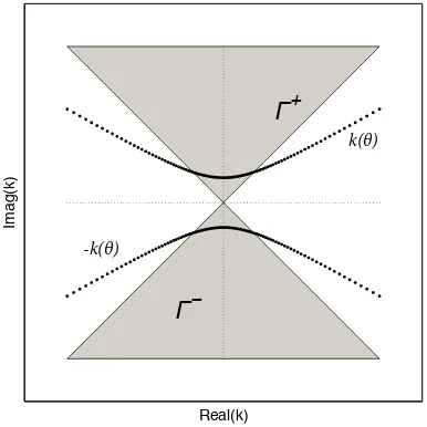
The analyticity of the functions involved in the integral representation of u(j)(x, τ) in (37), allows the replacement of the real axis(−∞,∞)by other contours of integration in the complex plane. For this, let
Γ = {k∈C: Re(γjk2)<0}
={k∈C: arg(k)∈(π
4, 3π
4 )∪( 5π
4 , 7π
4 )}
and
Γ+= Γ∩C+, C+={k∈C:Im(k)>0},
Γ−= Γ∩C−, C−={k∈C:Im(k)<0}.
Then, it can be easily verified, that:
• eicjk(x−wj−1) (x−w
j−1>0)is bounded and analytic for Im(k)>0
• eicjk(x−wj) (x−w
j <0)is bounded and analytic for
Im(k)<0
• e−k2τ (t≥0)is bounded and analytic for Re(k2)≥0. Therefore, by using Cauchy’s Theorem and Jordan’s Lemma, the representation ofu(j)(x, τ) in (37) can be equivalently expressed as
u(j)(x, τ) = cj 2π
Z +∞
−∞
eicjkx−k2τ
b
f(j)(cjk)dk
− 1
2πcj
Z
∂Γ+
eicjk(x−wj−1)−k2τ
·[ue(xj)(wj−1, k2) +icjkue (j)(w
j−1, k2)]dk
− 1
2πcj
Z
∂Γ−
eicjk(x−wj)−k2τ
·[ue(xj)(wj, k2) +icjkue(j)(wj, k2)]dk .
(52)
It is known (cf. [17], [18]) that one approach to the numerical quadrature of the above integrals is to apply the trapezoid rule on suitable hyperbolic contours (see also [5], [12]). For this, we map the pointsθ on the real line to the points ±k(θ) of the complex plane by using the analytic function:
Evidently thek(θ)and−k(θ)curves, as shown in Figure 1 replace the integration paths ∂Γ+ and∂Γ− respectively.
Real(k)
Imag(k)
Γ
+Γ
−k(θ)
[image:5.595.71.264.96.289.2]-k(θ)
Fig. 1: The contours±k(θ)for numerical integration
Using the above parametrization, the solution (52) is written as
u(j)(x, τ) = cj 2π
Z +∞
−∞
eicjkx−k2τ
b
f(j)(cjk)dk
− 1
2πcj
Z +∞
−∞
eicjkθ(x−wj−1)−k2θτ
·[eu(xj)(wj−1, kθ2) +icjkθeu(j)(wj−1, k2θ)]k
0
θdkθ
− 1
2πcj
Z +∞ −∞
e−icjkθ(x−wj)−k2θτ
·[eu(xj)(wj, k2θ)−icjkθeu (j)(w
j, kθ2)]k0θdkθ ,
(54) for all j= 1,2, . . . , n+ 1, withk0θ to denote the derivative of k(θ), namely
k0θ= cos(β−iθ). (55) We point out that the corresponding to (38)-(40) integral representations of the solution can be easily derived by ap-plying the constrains (24) as well as the Neumann boundary conditions.
D. Evaluation of the Integrals
The first integral in equation (54) can be evaluated analyt-ically (see also [9]) since the f(j) is a sum of Dirac’s delta functions. To be more specific, observe that
f(j)(x) = M
X
i=1
δ(x−ξi), for all ξi∈(wj−1, wj) (56)
hence
b
f(j)(cjk) = M
X
i=1
e−icjkξi, for all ξ
i∈(wj−1, wj) (57)
and therefore the first integral term in (54)
cj 2π
∞
Z
−∞
eicjkxe−k2τ
b
f(j)(cjk)dk=
cj
2√tπ
M
X
i=1 e−
c2j(ξi−x)2 4t .
(58)
The last two integrals in equation (54) have to be evaluated numerically. For the efficient implementation of numerical quadrature rules, one has to take into consideration the following basic algebraic properties:
• The real parts of all integrands areevenfunctions ofθ.
• The imaginary parts of all integrands areodd functions ofθ.
• The integrands are decaying functions ofθ.
The proof of the first two properties follows after a few algebraic manipulations (cf. [11]) while the third one is a direct consequence of the selected integration paths. Application of the above properties directly implies that
∞
Z
−∞
U(θ)dθ= 2
∞
Z
0
Re(U(θ))dθ≈2
Θ Z
0
Re(U(θ))dθ ,
where U(θ) denotes any one of the last two integrands involved in (54) and Θ is a relatively small real number. For a good estimate of Θ one may require the dominant exponential terme−k2θτ, common in all integrals, to satisfy
e
−k2θτ ≤10
−M for all θ≥Θ≡Θ(τ;M)
for sufficiently largeM, hence (cf. [9])
Θ = 1 2ln
4τ+ 8Mln 10
τ . (59)
NUMERICALSOLUTION
Following ( [5], [12]) and our work in [9], to numeri-cally evaluate the integrals in relation (54) above, we apply the trapezoid rule using the parametrization (53). For the asymptotes of the hyperbola withβ =π/6, as in [9].
For the numerical experiments we have used [a, b] = [−5,5]for the interval endpoints and
[w1, w2 , w3 , w4 , w5] = [−3, −2, −1, 0, 3]
for the interior interfaces. Cell motility and proliferation, in this artificial example, are using χ(t) = 0.2t, γj = γ =
Dg/Dw= 0.2 for allj= 1,3,5 andρ= 1.
x
-5 -4 -3 -2 -1 0 1 2 3 4 5
c
(
x
;t
)
[image:5.595.310.546.526.715.2]-5 0 5 10 15 20 25
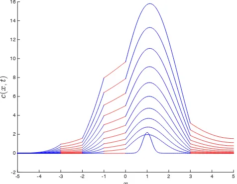
Fig. 2: Time evolution of cell densityc(x, t)for the case of two initial sources.
ξ2 = 1, is depicted for various time levels t = tm (m = 0,1, . . .). Hence, each curve on the figure represents the cell density at a specific time level, namelyc(x, tm). In complete analogy, in Figures 3 we depict the case of one initial source of cells centered, obsiously, atξ1= 1.
x
-5 -4 -3 -2 -1 0 1 2 3 4 5
c
(
x
;t
)
[image:6.595.51.289.141.326.2]-2 0 2 4 6 8 10 12 14 16
Fig. 3: Time evolution of cell densityc(x, t)for the case of one initial source.
Observe that, in both cases, the solution is continuous on the whole interval and smooth everywhere except at the interface points, as expected. We point out that, for the evaluation of each c(x, tm) curve no information at different time levels is used.
The relative error is given by
EN :=kuNi+1−uNik∞/kuNi+1k∞,
whereN denotes the number of quadrature points, and uN
is the corresponding numerical solution. From Figure 4 we observe the rapidly decaying convergence rate of EN.
Qudrature PointsN
0 20 40 60 80 100 120 140
E
rr
o
r
EN
10-16 10-14
10-12
10-10 10-8
10-6
10-4
10-2
Fig. 4: The relative errorEN
CONCLUSION
The Fokas transform method, combined with numerical integration on hyperbolic contours, is applied to the solution
of a multi-domain brain tumor invasion problem, modeled by a reaction-diffusion linear equation with time dependent coefficients and a discontinuous diffusion to characterize brain’s tissue heterogeneity. The exact solution is produced in integral form at any space-time point and evaluated by a fast convergent quadrature.
ACKNOWLEDGEMENT
The present research work has been co-financed by the European Union (European Social Fund ESF) and Greek national funds through the Operational Program Education and Lifelong Learning of the National Strategic Reference Framework (NSRF) - Research Funding Program: THALES (Grant number: MIS-379416). Investing in knowledge soci-ety through the European Social Fund.
REFERENCES
[1] Asvestas M, Sifalakis AG, Papadopoulou EP and Saridakis YS (2014) Fokas method for a multi-domain linear reaction-diffusion equation with discontinuous diffusivity, IOP Science Journal of Physics: Conference Series, 490, 012143.
[2] Cook J, Woodward DE, Tracqui P and Murray JD (1995)Resection of gliomas and life expectancy, J Neurooncol., 24, 131.
[3] Fokas AS (1997) A unified transform method for solving linear and certain nonlinear PDEs, Proc.R.Soc. A, 453, 1411-1443.
[4] Fokas AS (2002)A new transform method for evolution PDEs, IMA J. Appl. Math.,67(6), 559-590.
[5] Flyer N and Fokas AS (2008)A hybrid analytical-numerical method for solving evolution partial differential equations I: The half-line, Proc. R. Soc. A, 464, 1823-1849.
[6] Harpold HLP , Alvord Jr EC and Swanson KR (2007)The Evolution of Mathematical Modeling of Glioma Proliferation and Invasion, J Neuropathol Exp Neurol, 66(1), 1-9.
[7] Ledzewicz U, Schttler H, Friedman A and Kashdan E (2012) Math-ematical Methods and Models in Biomedicine, Springer Science and Business Media.
[8] Mandonnet E, Delattre J-Y, Tanguy M-L, Swanson KR, Carpentier AF, Duffau H, Cornu P, Van Effenterre R, Alvord EC, Capelle L (2003) Continuous Growth of Mean Tumor Diameter in a Subset of Grade II Gliomas, Ann Neurol, 53, 524528.
[9] Mantzavinos D, Papadomanolaki MG, Saridakis YG and Sifalakis AG (2014)A novel transform approach for a brain tumor invasion model with heterogeneous diffusion in 1+1 dimensions, Applied Numerical Mathematics (http://dx.doi.org/10.1016/j.apnum.2014.09.006). [10] Murray JD (2002)Mathematical Biology, Springer-Verlag.
[11] Papadomanolaki MG (2012)The collocation method for parabolic differential equations with discontinuous diffusion coefficient: in the direction of brain tumour,PhD Thesis, Technical University of Crete. [12] Papatheodorou TS and Kandili AN (2009)Novel numerical techniques
based on Fokas transforms, for the solution of initial boundary value problems, Journal of Computational and Applied Mathematics 227:75-82.
[13] D.A. Smith (2012)Well-posed two-point initial-boundary value prob-lems with arbitrary boundary conditions, Math. Proc. Camb. Philos. Soc. 152:473496.
[14] Swanson KR (1999)Mathematical modeling of the growth and control of tumors, PHD Thesis, University of Washington.
[15] Swanson KR, Alvord EC Jr and Murray JD (2000) A quantitive model for differential motility of gliomas in grey and white matter, Cell Proliferation, 33, 317-329.
[16] Tracqui P, Cruywagen GC, Woodward DE, Bartoo GT, Murray JD, Alvord Jr EC (1995)A mathematical model of glioma growth: the effect of chemotherapy on spatio-temporal growth, Cell Prolif, 28 1731. [17] Trefethen LN , Weideman JAC, Schmelzer T (2006)Tablot
quadra-tures and rational approximations, BIT Numerical Mathematics, 46:653-670.