Munich Personal RePEc Archive
Efficient Microlending without Joint
Liability
Altınok, Ahmet and Sever, Can
11 May 2014
Online at
https://mpra.ub.uni-muenchen.de/56598/
Efficient Microlending without Joint Liability
Ahmet Altınok∗ Can Sever†
June 11, 2014
Abstract
Peer-group mechanisms have been widely used by micro-credit institutions to minimize default risk. However, there are costs associated with establishing and maintaining liability groups. In the case when output is fully observable, we propose a dynamic individual lending mechanism. Assuming that risky borrowers discount the future costs and benefits relatively higher, our mechanism performs equally well in repayment rates, distinguishes safe and risky borrowers through differentiated interest rates and payment schedules. In case of unobservable types, it is able to eliminate adverse selection problem, and it reaches the first best outcome of the case that types of borrowers are publicly known. It improves wealth of individuals, and hence achieves a net welfare-superior outcome when compared with joint liability. Individual lending further saves from internal costs of group formation, and broadens the fractions of society into which microfinance institutions penetrate. We also identify unique welfare maximizing contract in our mechanism. Finally, we introduce a history dependent success probabilities, and show existence of efficient individual contract in that environment.
Keywords: Microfinance, Graamen bank, joint liability, adverse selection, microlending, group lending, individual lending
JEL Classification Numbers:
∗Address: Bo˘gazi¸ci University, Department of Economics, Natuk Birkan Building, 34342 Bebek, Istanbul,
(Turkey). e-mail: [email protected].
†Istanbul, (Turkey). e-mail:
1
Introduction
Microfinance institutions (MFI) mostly rely on joint liability (JL) mechanisms and peer-group effects to minimize the risk, reduce monitoring costs and achieve high turnout rates (Yunus, 1999). Participants are required to form a liability group (of varying sizes) to be eligible for a credit. It is argued that this innovation was instrumental in microfinance’s success (Armendariz de Aghion and Morduch, 2010; Daley-Harris, 2009; Morduch, 1999) and provide social collateral. Empirical evidence on that is mixed though. Al-Azzam et al. (2012) documented evidence for positive effects of peer monitoring on repayment rates. Attanasio et al. (2011), Gine and Karlan (2014) and Godquin (2007) found that the repayment rate does not significantly differ between individual and group lending. Wydick (1999) also found that group pres-sure is not significant in dealing with moral hazard. Gine et al. (2006) observed that ”the group-based mechanisms that are frequently employed can induce moral hazard (or more risk-taking behavior) instead of reducing it.”. Benarjee (2013) also argues about that the theory is missing that monitoring the others with no control on them increases free riding of others safe choices, and increase risk taking. Fischer (2010) with an experiment also concludes that JL stimulates risk taking further. Thus, we conclude that a model of group lending withex antetypes may fail to capture this effect of altering behaviors of individuals after group formation. With this in hand, we also know that Graamen, ACCION and BancoSol have been the pioneers of the group lending with different mechanisms, whereas, now they are converting from group to individual lending. The trend is same for Europe, El Salvador, Peru and many other countries.
There are potential sources of inefficiencies pertaining the group lending mechanisms. Group require-ment could cause an inefficiency by leaving out those who would have succeeded in availability of credit but do not have access to it because they couldn’t form a group1. Indeed, Gine and Karlan (2014) found that ”The conversion to individual liability did lead to larger lending groups, hence further outreach”(82). Furthermore, microcredit institutions offer a single loan scheme with a flat interest rate to all borrowers. However, both within groups and across groups, debtors differ in ability and potential to succeed. If credits were offered to individuals, adverse selection could be the result. Peer-groups are meant to induce cooperative behavior and keep turnout high. But there are costs associated with forming and maintaining groups, which raises an efficiency concern. Bhatta and Tang (1998) also mention about that in some cases MFI also involves in group formation mechanism which adds more administrative costs to the institution. Several studies investigated properties of joint-liability mechanisms. Besley and Coate (1995) showed that JL schemes may have positive and negative effects on repayment rates. Successful members will have an incentive to cover for those who couldn’t pay back. Liability works in other way if the whole group defaults (”strategic default”). Armendariz de Aghion (1999) showed that individual lending could outper-form group lending if peer monitoring is very costly and social sanctioning abilities are limited. Another problem Besley and Coate (1995) points to is collusion among borrowers in group lending, which demands more complex punishment mechanisms with potentially further monitoring costs. Our mechanism replaces individual liability while maintaining same expected return for the bank. So, it does not suffer from po-tential drawbacks of group liability.
Another strand of studies argue about the efficiency of JL and societal characteristics. Aghion and Morduch (2000) infer that group lending may be a poor mechanism for the industrialized societies. Lad-man and Acfha (1990) and Arene (1993) conclude that lack of cooperative behavior among members of the society give rise to failures of gruop lending in Bolivia and Nigeria, respectively. Moreover, Gine et al (2011) effect on religion on repayment rates of group lending. Ahlin and Townsend (2007) shows that social structures that decrease penalties may reduce the repayment. Cassaret al. (2007) and Azzamet al.
(2011) infer that the specific nature of society affects repayment performance differently. The latter found
that percentage of relatives in group may worsen the repayment rate, since it is hard to enforce relatives in some socities. These require a stirct analysis of the traditions and life style of the society in designing group mechanism which does not seem very practical. Bhatt and Tang (1998) emphasize the effect of geographic proximity on the success of group lending due to potentially high costs of communication and monitoring of peers. Noballa (1992) and Azzamet al. (2011) represent the evidence of this kind of negative impacts. Addilitonally, JL in general depends on that ex-ante borrowers know each others types which is a hidden information in terms of banks. This assumption is even harder to the members who are not geographically close. All these reveal the difficulties for implementing ”true” group lending mechanism for different societies, and thus pave the way for individual lending.
For borrowers’ side, group formation costly, internal cost of this. The amount of this cost may prevent the borrower to go to bank and it depends on the social environment she has. If they do not know each other for a long time, they may not have an idea about the risk of the others projects, which is assumed in theory. and they cannot trust. Also as discussed, Close relatives cannot apply sanctions to each others in some societies.
Rai and Sjostrom (2004) argued that a JL mechanism with a cross-reporting scheme leads to a better risk-sharing and less defaults. Bhole and Ogden (2010) similarly discussed the importance of cross-reporting mechanisms and found that in the absence of sanctions, group lending does worse than individual lending in repayment rates. Bond and Rai (2008) relied on social sanctions to enforce payments. Given the costly nature of such sanctions, it would be an improvement if we can substitute individual liability instead of group liability while maintaining same returns. Our dynamic mechanism addresses this problem. Bond and Rai (2008) proposes “cosigned loans” as an alternative to group loans when sanctioning abilities differ among individuals. Our individual lending mechanism produces better results in terms of welfare than JL schemes, independent of sanctioning abilities.
Individual lending as an alternative to group-lending were not studied as extensively as group lend-ing mechanisms. One notable exception is Armendariz de Aghion and Morduch (2000). They propose mechanisms with more stringent direct monitoring and restricted payment schedules that brings an effect equivalent to peer groups. Assuming that riskier types discount the future more, our mechanism introduces differentiating interest rates and repayment schedules which achieves same outcome without further direct monitoring.
Bhatt and Tang (1998) extensively discusses transaction costs in group lending. They point to the ”...costs associated with screening potential group members, group formation, agreeing on formal or infor-mal group rules...” (624). Shatragom and Bayer (2013) argues in similar vein. The mechanism we develop addresses transaction cost concerns in two ways. We require no group formation so there is no fixed cost of eligibility. Also in equilibrium, the loan contract that bank offers leads to a self-selection of agents (safe and risky types) with respect to their success probabilities. This differentiation reduces bank’s monitoring costs and improves welfare.
extends the reach of credit opportunities by relaxing the group requirement. Benarjee (2013) addresses the new directions for future reseach on theoretical side. He discusses the significance of identifying optimal dynamic credit contract under the presence of behavioral aspects. In line with Banerjee (2013)’s agenda, we also investigate the impact of JL in dynamic contracts and show that individual liability mechanism we offer strictly dominates an equivalent JL mechanism in terms of welfare. The dynamic aspects of our mechanism are essential. In the practice, microfinance institutions sign a dynamic repayment scheme with their borrowers in weekly or monthly terms. In many practical cases, payments starts in general as soon as borrowing is done in the following week or month. Fischer (2011) hints that just a 2 month delay for repayment makes a large effect on income of borrowers. Indeed, the wedge between discount factors allowed a welfare-superior individual liability credit contract. Ghatak and Guinnane (1999) and Chowdhury (2005, 2007) work in sequential environments. In our dynamic model, we assume that output realizations occur every period and borrowers discount future. In case of that types of borrowers are not private information by the lender, there is no problem and bank can charge perfectly desired interest rates to each type. This yields the first best outcome with distinct rates for distinct types. On the other side, if it cannot observe the types of borrowers, a unique contract may pose adverse selection problem. We assume types of agents are not seen by lender, and differentiate the payment schemes. We introduce two schemes and first alter period-wise payments of only one type of contract. Using our assumption that safe type discounts less than risky type, we solve adverse selection problem. Hence, we achieve exactly to the best outcome in which types are observed by the bank. We also improve welfare of both individuals and society when compared with the JL case in which bank gets same expected repayment. Second, we also alter the other contract and introduce a new payment scheme which further increase individual welfares. It is also the welfare-maximizing contracts for the society. We finally extend our environment to a more general one. We relax the history independent success probabilities, and add a memory to the likelihood of success of projects. In this new environment, we also show the existence of same kind of contract with individual lending. To the best of our knowledge, this study is the first in the microlending literature, by incorporating dynamic payment scheme and discount factors of individuals, which at the end reaches the first best solution with individual lending mechanism.
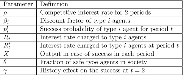
Our mechanism screens safe and risky types under an individual lending scheme without a loss to the bank and society. Ghatak (1999,2000) showed that with JL and self-selection, safe borrowers gather to-gether to form credit cooperatives and risky borrowers are screened out. We achieve the same equilibrium outcome without JL. Ghatak and Guinnane (1999) discusses moral hazard problems in group-lending. We’ve already discussed the cost issues of such peer-monitoring mechanisms. Thus, there is a clear effi-ciency gain from replacing JL with individual liability in case of observable outputs.Table 1 represents the summary of parameters.
Parameter Definition
ρ Competetive interest rate for 2 periods
βi Discount factor of type iagents
pt
i Success probability of type iagent for periodt
Ri Interest rate charged to typei agents
Ri
t Interest rate charged to typei agents at periodt
X Output in case of success in each period
θ Fraction of safe tyoe agents in society
[image:5.612.153.462.534.662.2]γ History effect on the success att= 2
The rest of the paper is organized as follows: Section 2 introduces the model. Section 3 introduces the benchmark individual contract shceme with welfare discussions. Section 4 identifies the welfare maximizing one among these individual contracts. Finally, in Section 5, we change the environment with history dependency and identify the contract in this environment. Section 6 concludes.
2
Model
There are two types of potential borrowers, safe and risky. θ fraction of all borrowers are of safe type whereas (1−θ) fraction of them are risky. Types are private information of each borrowers herself. Neithr other borrowers nor the lender does not know the type of any borrower. Each type borrows from the same lender (MFI), and invest their funds in their businesses. We assume output for projects are same regardless of types. Investment of each borrower either yields a revenue of X with a positive probability or nothing for each period. Hence, if a borrower succeeds for both periods, she receives 2X as output. We assume that the lender observes this output for each period. Following Rai and Sjstrm (2004), we assume poor people have no assets, then they are not supposed to repay anything in case of failure. Borrowers are required to pay (gross) interest on their loan only when the outcome is success. Letps and pr be the
success probabilities of safe and risky types, respectively and for each period. We assume that ps> pr.
Let ρ be the two-period market interest rate, which is defined as the total amount a borrower need to pay back for $1 credit. Following Rai and Sjostrom (2004), we assume that microcredit institution in a competetive market sets interest ratesR such that the expected revenue is market rate. This may be also called as zero profit constraint (ZPC) for MFI. Thus, it does not extract profit for itself, and supposed to maximize welfare of society. In the case of a uniform credit contract, this corresponds to pR =ρ where
p=θps+ (1−θ)pr (i.e. average success probability for the society). Let Rs and Rr be the interest bank
is willing to charge to safe and risky types, respectively if it can observe the types. That is, there rates are able to perfectly differentiate the types and there is no adverse selection problem. Then, ZPC implies
psRs =prRr =pR=ρ. We note that since ps> pr,Rs< Rr.
We construct a dynamic framework in which agents borrow in period 0, invest in their businesses and repay the interest in two (not necessarily equal) periodic installments. Ri
t denotes the payment type i is
[image:6.612.121.489.470.629.2]supposed to make at time taccording to her contract. Following diagram illustrates the timeline:
Figure 1: Timeline
village economy, and try to sell those. Having made the investment, the probability that she can sell her products is approximtely same for each time period. Agents are risk-neutral. In a given period, net utility of a borrower type i is pi(X −Rit). Safe and risky borrowers discount future benefits with βs and βr
respectively. We assume that βs ≥ βr, which is, as we will show, a necessary condition for existence of
differentiated contracts that are incentive compatible. One can interpret this as follows: safe individuals are more likely succeed in future periods so they tend be concerned less about immediate gratification. With these in hand, expected utility of agent iwith individual contract (Hi
1, H2i) as follows:
EUi(H1i, H2i) =piβi(X−H1i) +piβi2(X−H2i) ∀ i∈ {s, r}
Given the fraction of safe types in the society θ and payment schemes for both type (H1s, H2s) and (Hr
1, H2r), welfare of the society is given as follows:
EWsoc(H1s, H2s, H1r, H2r) =θ(psβs(X−H1s) +psβs2(X−H2s))+
(1−θ)(prβr(X−H1r) +prβ2r(X−H2r))
Given that types are not observable and psRs=prRr =pR=ρ, if agents were not to discount future
benefits and costs, safe type’s contract has strictly better terms. Both types would prefer safe type’s contract. It creates the adverse selection problem in static environment, and gives incetive to the bank to charge a global rate R. Eventually, since Rs < R < Rr, safe types are worse off and risky types are
better off. In what follows, in dynamic environment, we will demonstrate that, if βs ≥ βr, there exists
an incentive compatible contract scheme such that agents of each type prefer their own contracts (agents are screened according to their types). We also show that such a scheme requires Rs
1 > Rs2. Intuitively,
we exploit the difference between discount factors. By sufficiently increasing the early installment of safe type’s contract, it is possible to make it unattractive to risky type even though Rr> Rs, i.e. risky type’s
contract requires a higher undiscounted total payment. Later, we show the welfare gain of our individual lending mechanism over the corresponding JL schemes.
3
Dynamic Contract with Observable Output
We now propose a dynamic contracting mechanism which addresses hidden types i.e. the adverse selection issue. Initially, we will fix risky types repayment scheme {Rr
1, Rr2} = {R2r,
Rr
2 }, i.e. a standard
repayment schedule in practice, and establish the existence of {Rs
1, Rs2} that satisfies the requirements
provided in the following proposition.
Without loss of generality, we fix outside option to 0 for all types. Hence, individual rationality constraints for safe and risky types are as follows:
IR(s) :EUs(Rs1, Rs2)≥0 (1)
IR(r) :EUr(R1r, Rr2)≥0 (2)
Solving IR’s of both types we get the minimum level of output:
X ≥ R
s
1(1−βs) +βsRs
X ≥ Rr
2 We endogenously get Rr
2 ≤ X which is the condition that period-wise payment for risky type cannot
be greater than period-wise payment. It is also received in aggregate terms for risky type. In addition, since Rs < Rr, the result in aggregate terms is valid for safe type, too. We additionally assume X ≥Rst
fort= 1,2, since poor people are assumed to have no endownments. We also need incentive compatibility constraints to induce each agent to prefer the credit contract suited for her own type:
IC(s) :EUs(R1s, Rs2)≥EUs(Rr1, Rr2) (3)
IC(r) :EUr(Rr1, R2r)≥EUr(R1s, Rs2) (4)
where we fix Rr
t = R2r in the contract as in most of real-world contracts. We only allow to choose the
reallocation of safe type’s payment scheme. By solving these IC’s,
ps
2pr(1 +βs)−βs
1−βs
Rs≥R1s≥
ps
2pr(1 +βr)−βr
1−βr
Rs (5)
As long asβs≥βr, there existsRs1which can implement the contract. The consequences are represented
in following proposition.
Proposition 1 For all βi, pi ∈ (0,1), βs ≥ βr and ps > pr with sufficiently large output level X, there
exists a two-period repayment schedule {Rs
1, R2s, Rr1, Rr2} s.t.
1. {Rr1, Rr2}={R2r,R2r}
2. Safe type agents prefer {Rs
1, R2s}
3. Risky type agents prefer {Rr
1, Rr2}
4. Bank’s expected revenue from both type is the same
where Rs
1 satisfies (5), and Rs2 =Rs−Rs1 with ZPC.
Proof. See appendix.
Proposition 1 shows the existence of a contracting scheme that screens agents according to their types. We note that MFI can implement this scheme with only chosing one variable Rs
1. In the next section, we
investigate the welfare properties of this mechanism. We also note that the case βs =βr, the contract is
unique. We also note that there may be cases in whichRs
1 > Rs. This means safe type may pay more than
total amount in the first period, then she receives some amount back at the final period. Our assumption
X > Rs
1 makes this kind of situation possible. On the other hand, there is an upper bound for βr which
gives rise to that Rs
1 ≤Rs always holds2.
We now turn to welfare issues. In what follows, we first show that our becnhmark payment interval maximizes the expected welfare of th society when we setRs
1 ot its lower bound. By doing so, we receive
the maximum welfare case of our becnhmark contract. We then compare the differentiated repayment schemes we propose is superior to JL contracts in terms of both social and individual welfares.
Claim: Rs∗
1 = ps
2pr(1+βr)−βr
1−βr Rs must be the choice in the benchmark contract in order to get the
maximal level of safe type utility, and hence maximize the societal welfare. Since societal welfare in this case is as follows,
EWsoc(R1s, Rs2,
Rr
2 ,
Rr
2 ) =θpsβs((βs+ 1)X−βsRs+ (βs−1)R
s
1)
+(1−θ)prβr((βr+ 1)X−Rr
βr+ 1
2 )
Since βs < 1, the minimal value of Rs1 the one that maximizes the expected utility of the safe type.
Due to uniform scheme of risky type, it is also welfare maximizing choice for the society.
3.1 Individual vs. Joint Liability
Since our contract has the ability to differentiate types as in the case that types are common knowloedge, it improves the wealth when compared with the uniform contract with (R1, R2) and whereR1+R2 =R.
An alternative mechanism could make use of JL within a dynamic contract.
In JL, positive assortive matching is one possibility. Ghatak (1999) and van Tassel (1999) argue that it is more likely to occur in static environment. Moreover, the socially optimal matching may change in dynamic environment. Thus, we are not sure which is the welfare superior. As a result we take both cases of JL into account. In a 2-person group scheme, expected welfare of typeiwhen she borrows with a group of j type is given as follows:
EUiJ L(R1i, R2i, j) =pipjβi(X−Ri1) +pi(1−pj)βi(X−Ri1−R
j
1) (6)
+pipjβ2i(X−Ri1) +pi(1−pj)βi2(X−R2i −Rj2) (7)
where j is type of her peer in the group. Positive assortive matching means j =i, whereas, negative asortive matching is thatjandiare different types. As a result, social welfare in case of a general matching of iand j types is defined as follows:
EWsocJ L(R1i, R2i, R1j, R2j, i, j) =θi(pipjβi(X−Ri1) +pi(1−pj)βi(X−Ri1−Rj1) (8)
+pipjβi2(X−Ri1) +pi(1−pj)βi2(X−Ri2−Rj2))+ (9)
(1−θi)(pjpiβj(X−Rj1) +pj(1−pi)βj(X−Rj1−R1i) (10)
+pjpiβj2(X−R j
1) +pj(1−pi)βj2(X−R j
2−Ri2)) (11)
where θi is the fraction of i tyoe in the society. On the other hand, following proposition shows that
individual lending is welfare-superior to both cases of group lending.
Proposition 2 For a given periodic repayment dynamic contract with differing time preferences of bor-rowers, individual liability credit scheme provided in Proposition 1 welfare dominates a JL scheme both individually and socially.
Proof. See Appendix.
an environment where output is observable, JL mechanisms could be used to address adverse selection issues. However, the difference in time preferences allow us to construct a pair of contracts such that each agent self-selects herself to the contract suitable for her type. Implementing JL in this context brings no improvement in selection while burdening each agent with a partner’s risks. Hence, individual liability mechanisms are superior in welfare4. We also illustrate the result with an example of initial parameters.
Example 1: In this example we show that our benchmark contract with payment scheme (Rs∗
1 , Rs2∗,R2r,
Rr 2 )
improves welfare both individually and thus societally when compared with positive (i, i) and negative (i, j) assortive matching cases of JL. Exogenous parameters are (θ, ps, pr, ρ, βr, βs, X),
Exogenous parameters
βs βr ρ pr ps X θ
0.9 0.7 1.05 0.7 0.8 1.2 0.6
UsingpsRs=prRr=pR=ρ, we calculate endogenous parameters,
Endogenous paramters
R Rs Rr p
1.3816 1.3125 1.5000 0.7600
Then selecting benchmark contract for safe types in case of individual liability to maximize societal welfare, we calculate Rs∗
1 = 1.1875, thus Rs2∗ = 0.1250. We also note that Rr1 =R2r. With these in hand,
we calcaluate and compare welfares with the JL in case of both types of matchings.
Welfare Individual contract JL (i, i) matching JL (i, j) matching
Society 0.5735 0.3860 0.3386
Safe agent 0.7059 0.5184 0.3978
Risky agent 0.3749 0.1874 0.2499
As illustrated, individual contract scheme we proposed improves the welfare in significant levels. In our scheme society has expected welfare as 0.5735, whereas the levels are 0.3860 and 0.3386 in positive and negative assortive matching cases respectively of gruop lending with full liaibility. Additionally, individual based utilities areex antr increased for both types. Safe type agent receives 0.7059 in our scheme, whereas she gets 0.5184 in maximal case of JL. The result is valid by comparing individual vs group lending with numbers 0.3749 and 0.2499, respectively. The impact of individual improvements on the societal increase depends on the composition of society i.e. θ. Moreover, the effect of the individual contract on each type is related to theirpi and βi values.
4
The Contract with Welfare Evaluations
So far we restricted ourselves the optimal choice of safe type’s contract {Rs
1, Rs2} keeping {Rr1, R2r}= {R2r,R2r}. We demonstrated the welfare gain associated with differentiating safe type’s contract. Now we
4Indeed, as argued in introduction, there are further transaction costs associated with JL mechanisms which we do not
let Rr
1 6= Rr2, so the problem becomes choosing {Rr1, R1s}. Since Ri2 =Ri−Ri1, we do not count them as
choice variables. Following proposition characterizes the new pair of efficient contracts and then get the ones that are welfare maxizing. We again have same IC and IR constraints, but not with Rr
2 but with
(Rr
1, Rr2). Solving those we get following restrictions:
X ≥ R
i
1(1−βi) +βiRi
1−βi
∀ i∈ {s, r}
Rs
βr(pprs −1)
1−βr
≤Rs1−Rr1≤Rs
βs(ppsr −1)
1−βs
As long as βs≥βr, the contract is pmlementable. Following proposition states that it can be different
from our benchmark contracting scheme.
Proposition 3 For all pi, βi∈(0,1)andβs≥βr withps> pr with sufficiently large output level X, there
exists a two-period repayment schedule {R1s, Rs2, Rr1, Rr2} s.t. condition in Proposition 1 are satisfied and
{Rs
1, R2s} is not necessarily {Rr/2, Rr/2}
Proof. See Appendix.
We also note that the case βs = βr, the contract is unique. The merit of flexibility in both types’
contracts becomes apparent when we consider the welfare improvement. The societal welfare can be rewritten as:
EWsoc(Rs1, Rs2, Rr1, R2r) =K+θpsβs(βs−1)Rs
(1 +βr)2ppsr −βr
1−βr
+ (1−θ)prβr(βr−1)
Rr
2
where K=θpsβs(1 +βs)X−θpsβs2Rs+ (1−θ)prβr(1 +βr)X−(1−θ)prβr2Rr.
As can be seen, we have negative coefficients with Rs
1 and Rr1, and restriction containing difference of
the two. By taking Rr
1 = 0, and also setting minimum Rs1, we maximize the societal welfare, as well as
that of individuals. Following proposition represents the result.
Proposition 4 Fully differentiated contract pair with {Rs∗
1 , Rs2∗, Rr1∗, Rr2∗} yields the maximum welfare
both individually and socially, where Rr∗
1 = 0 and Rs1∗ = Rs βr(ps
pr−1)
1−βr . From ZPC, payments at t = 2 is
found by Ri
2 =Ri−Ri1 for both types.
Proof. See Appendix.
Thus, allowing one type contract with payment only at t = 2, and reallocating the other compared with benchmark contract, we identify the welfare maximizing one for both individuals and the society. Proposition 4 implies that it is possible to improve welfare further if we allow risky type’s contract to have varying period installments. In practice, it is common among microcredit institutions to demand uniform installments. Our result, however, suggests otherwise in the presence of heterogeneous time preferences. We illutrate welfare increase with an example of benchmark paramaters:
Example 2: We illustrate that our new contract (withRr
1 choice) further improve the welfare in both
Welfare Contract with (Rs∗
1 , Rr1∗) Benchmark contract
Society 0.6498 0.5735
Safe 0.7596 0.7059
Risky 0.4851 0.3749
We observe that for this set of parameters, ex antesocietal welfare jumps from 0.5735 to 0.6498 with this further choice in the contracting scheme. Moreover, both risky and safe types receive increases in their utilities as 0.0537 and 0.1102, respectively. We note that relative levels of individual welfare improvements depend onpi and βi values. In addition,θ determines the effect of individual enhancements on the overall
improvement of welfare.
5
History dependent probabilities
We now turn our attention into a scenario in which the outcome of the first period -being either success or fail- has an affect on the probability of success in the second period. This is an attempt to introduce a more realistic model. We define γ as the memory dependence of the projects of both types. At t = 2, the probability of success and fail for each type is now conditional on the outcome att= 1. We introduce symmetric effect of past on t= 2 with γ. Now p1,i =6 p2,i there pt,i is the success probability of type iat
timet. If agent of type isucceeds att= 1,p2,i=p1,i+γ, otherwise, it isp2,i =p1,i−γ. Thus the nature
of dependency is same for each type and bad or good news from period 1 affects in same amount.
The second periods probabilty of success is now kind of an expected probability of success for either type, and it is equal topi
2 = 2pi1γ+pi1−γ. We can also summarize these like below:
p2,i(Success at t= 2|Success at t= 1) =p1,i+γ
p2,i(Success at t= 2|F ailure at t= 1) =p1,i−γ
Note that ps > pr implies ps,2 > pr,2. In this environment, expected utility of agent type i is the
following:
EUi=βipi(X−Rs1) +βi2(pi(pi+γ) + (1−pi)(pi−γ))(X−Ri2) (12)
This extension alters ZPC of bank, and IR’s as well as IC constraints of the individuals. Here is ZPC of the bank with this manipulation:
piRi1+ (pi(pi+γ) + (1−pi)(pi−γ))Rs2 =ρ ∀ i ∈ {s, r} (13)
Solving ZPC above for both types gives the second periods’ repayment i.e.
Ri2 = (Ri−R
i
1)pi
2γpi+pi−γ
IR(s):
psβs(X−Rs1) +βs2(2psγ+ps−γ)
| {z }
ps,2
(X−Rs2)≥0
IR(r):
prβr(X−Rr1) +βr2(2prγ+pr−γ)
| {z }
pr,2
Solving the individual rationality constraints above gives a lower bound for the level of outputX :
X ≥ piR
i
1+Ri2(2piγβi+piβi−γ)
pi+piβi+ 2piγβi−γ
(14)
whereRi
2=
(Ri−Ri1)pi 2γpi+pi−γ.
The new incentive compatibility constraints are now;
IC(s):
psβs(X−Rs1) +βs2(2psγ+ps−γ)Rs2 ≥ psβs(X−Rr1) +βs2(2psγ+ps−γ)(X−Rr2)
IC(r):
prβr(X−Rr1) +βr2(2prγ+pr−γ)Rr2 ≥ prβr(X−R1s) +βr2(2prγ+pr−γ)(X−Rs2)
Note that the only difference from the previous incentive compatibility constraints is in the second periods’ probability of success. Following proposition states the existence of the efficient individual lending contracting schemes in this environment.
Proposition 5 For all pi, βi ∈ (0,1), ps > pr, and sufficiently large output level X, if history effect is
appropriate5, there exists a fully differentiated contract pair for both types; who has history dependent probabilities of success (ps,2, pr,2), which gives the maximum welfare both individually and societally.
Proof. Solving IC(s), andIC(r), above; gives
Rs1(1−βs)−Rr1(1 +
βsps,2pr
pr,2ps
)≤ βsρ(ps,2−pr,2)
pspr,2
Rs
1(1 +
βrpr,2ps
ps,2pr
)−Rr
1(1−βr)≥
βrρ(ps,2−pr,2)
prps,2
Note that, to be able to maximize social welfare which is
EW
′(Rs
1,Rs2,Rr1,Rr2)=θ(psβs(X−Rs1)+β2s(2psγ+ps−γ)R2s)+
soc
(1−θ) prβr(X−Rr1) +βr2(2prγ +pr−γ)Rr2
we need to takeRs
1 andRr1as small as possible6. ForIC(r) to be satisfied,Rs1should be nonzero, however,
Rr
1 = 0 poses no threat for the IC constraints. Now that we are sure, we can set Rr1 = 0 this gives new
boundaries forRs
1; which is;
βrρ(ps,2−pr,2)
prps,2
(1 + βrpr,2ps
ps,2pr )
≤Rs1≤
βsρ(ps,2−pr,2)
pspr,2
(1−βs)
As long as the upper bound is greater than the lower bound for Rs
1, we can ensure that there exists
a repayment schedule which deals with the adverse selection problem as well as maximizes social and
5We have some limitations onγ: 0≤γ,p
individual welfare. Need to show that
βrρ(ps,2−pr,2)
prps,2
(1 +βrpr,2ps
ps,2pr ) ≤
βsρ(ps,2−pr,2)
pspr,2
(1−βs)
By some algebra, we get
2βsβrpspr,2+βsps,2pr−βrpr,2ps ≥0
Note that, prps,2 ≥ pspr,2 implies the inequality above 7. This ensures that the upper bound of Rs1 is
strictly greater than the lower bound. Hence, we can choose Rs
1 as the lower bound which satisfies the
IC by construction and maximizes both social and individual welfare 8. Summing up all, the repayment schedule{Rs∗
1 , R2s∗, Rr1∗, Rr2∗}where
R1s∗ = βrρ(ps,2−pr,2)
ps,2pr+βrpr,2ps
Rs2∗= (Rs−R
s
1)ps
2γps+ps−γ
Rr∗
1 = 0
Rr2∗= Rrpr 2γpr+pr−γ
identify the optimal contract that solves adverse selection problem and maximizes the social welfare as well as that of individuals.
We note that, since period-wise success probabilities are not uniform in this environment. Ri t also
depends upon (pi
1, pi2), since the outcome of first period affects the second.
6
Conclusion
In this paper, we introduced a dynamic credit contract with individual lending to tackle adverse selection issues in micro-credits. We first assumed that output is fully observable to the lender and showed that in a dynamic setting, it is possible to formulate an individual lending scheme that screens safe and risky borrowers, generates the same expected revenue for the lender and improves welfare of the society. This has profound implications for the evolution of microcredit programs. There has been a shift from group lending to individual lending in many leading microcredit institutions (Armendariz de Aghion and Morduch 2005, 119-120). Given that forming and maintaining a peer group has transaction costs and the empirical evidence about its effectiveness is mixed, a switch to robust individual lending mechanisms should be desirable. We offer one such mechanism, based on the premise that borrowers have different time preferences.
Our mechanism perfectly screens borrowers with differentiated contracts. Bank is still equally likely to extend contracts to all sorts of borrowers, so the reach of credit is not harmed. Indeed, by saving from the costs associated to JL mechanisms, our mechanism is likely to extend the reach of credit opportunities. This is a very desirable result and in accordance with objectives of micro-credit programs.
7Easily it can be seen by pluggingp
i,2 intoprps,2> pspr,2 wherepi,2= (2piγ+pi−γ) for alli∈ {s, r}
8Note that,γ= 0 is the benchmark case which is consistent with the result here as long as safe type discounts less than
7
References
Al-Azzam, Moh’d, R. Carter Hill, Sudipta Sarangi. 2012. ”Repayment performance in group lending: Evidence from Jordan,”Journal of Development Economics, 97(2): 404-414.
Armendariz de Aghion, Beatriz. 1999. “On the design of a credit agreement with peer monitoring”.
Journal of Development Economics, 60: 79-104.
Armendariz de Aghion, Beatriz and Jonathan Morduch. 2000. “Microfinance beyond group lending”,
Economics of Transition, 8(2): 401-420.
Armendariz de Aghion, Beatriz and Jonathan Morduch. 2010. The Economics of Microfinance, 2nd ed. MIT Press, Cambridge, MA.
Attanasio, Orazio, Britta Augsburg, Ralph De Haas, Emla Fitzsimons, Heike Harmgart. 2011. ”Group lending or individual lending? Evidence from a randomised field experiment in Mongolia,” Working Papers 136, European Bank for Reconstruction and Development, Office
Banerjee, A. 2013. “Microcredit under the microscope: What have we learned in the past two decades, and what do we need to know?”, Annual Reviews of Economics, 5:487519.
Bayer, Ralph and Sujiphong Shatragom. 2013. The University of Adelaide School of Economics Re-search Paper No. 2013-23
Besley TJ, Coate S. 1995. “Group lending, repayment incentives and social collateral.” J. Dev. Econ, 46:118
Bhatt, Nitin and Shui-Yan Tang. 1998. “The Problem of Transaction Costs in Group-Based Microlend-ing: An Institutional Perspective”,World Development, 26(4): 623-637.
Bole, Bharat and Sean Ogden. 2010. “Group lending and individual lending with strategic default”,
Journal of Development Economics, 91: 348363
Bond P, Rai AS. 2008. “Cosigned vs. group loans.” J. Dev. Econ., 85:5880
Chowdhury, PR. 2005. “Group-lending: sequential financing, lender monitoring and joint liability.” J. Dev. Econ. 77:41539
Chowdhury, PR. 2007. “Group-lending with sequential financing, contingent renewal and social capi-tal”,Journal of Development Economics. 84:487506
Daley-Harris, 2009. “State of the Microcredit”, Summit Campaign Report, Washington, DC.
Fischer G. 2011. “Contract structure, risk sharing and investment choice”, Econ. Org. Public Policy Discuss. Pap. 023, Suntory Toyota Int. Cent. Econ. Related Discipl., London School Econ.
Ghatak M. 1999. “Group lending, local information and peer selection.” J. Dev. Econ., 60:2750 Ghatak M. 2000. “Screening by the company you keep: joint liability lending and the peer selection effect.” Econ. J., 110:60131
Ghatak M, Guinnane TW. 1999. “The economics of lending with joint liability: theory and practice.”
J. Dev. Econ., 60:195228
Gin X, Jakiela P, Karlan D, Morduch J. 2010. Microfinance games. Am. Econ. J. Appl. Econ.
2(3):6095
Gin, Xavier and Dean S. Karlan. 2014. “Group versus individual liability: Short and long term evi-dence from Philippine microcredit lending groups”,Journal of Development Economics, 107: 65-83
Morduch, Jonathan, 1999. The microfinance promise. J. Econ. Lit.. 37(4): 1569 - 1614.
Rai AS, Sjstrm T. 2004. Is Grameen lending efficient? Repayment incentives and insurance in village economies. Rev. Econ. Stud., 71:21734
Tassel V. E. 1999. ”Group lending under asymmetric information,” Journal of Economic Dynamics and Control, 60(1): 3-25.
lending in Guatemala. Economic Journal, 109:46375
Yunus, M. (1999), The Grameen Bank, Scientific American, 114 - 119.
8
Appendix
8.1 Proof of Proposition 1
Note that the expected utility of an agent is the following:
EUi(H1, H2) =piβi(X−H1) +piβi2(X−H2)∀i∈ {s, r}
where Ht is the payment scheme∀ t ∈ {1,2}. Recall that the bank sets it. For such a contract to exist,
need to see that there is an interval forR1sto be chosen, so that we can choose it and satisfy the conditions (with sufficiently largeXof course, to be able to satisfy agents to participate.) Remember, the boundaries coming from individual compatibility constraints are9:
ps
2pr(1 +βr)−βr
1−βr
Rs≤Rs1 ≤
ps
2pr(1 +βs)−βs
1−βs
Rs
and the lower boundary of the output levelX is either10
Rs1(1−βs) +βsRs
1 +βs
≤X or Rr 2 ≤X
With the assumption of the output levelXbeing sufficiently large, each agent’s contract yields nonnegative benefits in expected terms and which ensures participation. Therefore, Individual rationality constraints are not an issue here. As long as we can show that the upper bound is greater than the lower bound of
Rs
1, we are done. But, withβs≥βr and ps≥pr, one can easily see that; ps
2pr(1 +βr)−βr
1−βr
Rs≤ ps
2pr(1 +βs)−βs
1−βs
Rs
Hence, there existsRs
1that satisfy individual compatibility constraints. This basically completes the proof.
Now that, we claim
ps
2pr(1+βr)−βr 1−βr ≥
1 2.
ps
pr
(1 +βr)−2βr≥1−βr
ps
pr
(1 +βr)≥1 +βr ⇒Rs1 >
Rs
2 (15)
Also note that fromICr(4), if we assume the first instalmentRs1cannot be greater than the total repayment
Rs, then we will have an upper bound for risky types discounting which isβ
r≤ 2ppsr −1. However, it is not
that strict. We can also assume that the safe type borrower can pay more than the repayment at the first stage and get some back at the second stage.
9whereIC(s) :EU
8.2 Proof of Proposition 2
Under individual liability, we have
EUi(Ri1, R2i) =piβi(X−Ri1) +piβi2(X−Ri2) (16)
The joint liability contract yields the following utility for type iwho has the peer j,
EUiJ L(Ri1, Ri2, R1j, R2j, j) =pipjβi(X−Ri1) +pi(1−pj)βi(X−Ri1−Rj1)
+pipjβi2(X−Ri1) +pi(1−pj)β2i(X−Ri2−R
j
2)
Under joint liability, each borrower ihas to cover for her associate’s paymentRj in case of failure 11.
We need to show EUi()> EUiJ L()∀Ri, Rj ∈R++. The expression becomes:
pi(X−Ri1) +piβi(X−Ri2)>[pipj+pi(1−pj)](X−Ri1) +βi[pipj+pi(1−pj)](X−R2i) −pi(1−pj)Rj1−βipi(1−pj)R2j
Since pipj+pi(1−pj) =pi, this reduces to
pi(1−pj)Rj1+βipi(1−pj)Rj2>0
which is satisfied for sure.
8.3 Proof of Proposition 3
Here, rather than fixing Rr
1 to R2r, we choose both Rs1and Rr1 where they are the repayment in the
first period for the safe type and repayment in the first period for the risky type, respectively. From the ZPC, the secnd period’s repayment levels are determined. Under the light of this new set-up, individual rationality and incentive compatibility constraints, in the same order presented in Proposition 1, are the followings:
IR(s) :βsps(X−Rs1) +βs2ps(X−rs2)≥0
IR(r) :βrpr(X−Rr1) +βr2pr(X−R2r)≥0
IC(s) :βsps(X−Rs1) +βs2ps(X−R2s)≥βsps(X−R1r) +βs2ps(X−Rr2)
IC(r) :βrpr(X−Rr1) +βr2pr(X−R2r)≥βrpr(X−R1s) +βr2pr(X−Rs2)
We still have psRs = prRr = pR = ρ as the moneylender’s behaviour. Solving the participation
conditions i.e. IRs gives a new lower boundary for the output level X; which is
max
Rs
1(1−βs) +βsRs
(1 +βs)
,R
r
1(1−βr) +βrRr
(1 +βr)
11which occurs with probabilityp
After achieving the level of Output to satisfy the players participate in the mechanism, we need to lead either type to behave as themselves. Incentive Compatibility constraints capture this requirement. Hence, solving the last two inequality above yields;
Rs
βr(pprs −1)
1−βr
≤Rs1−Rr1≤Rs
βs(ppsr −1)
1−βs
Here again, since the both boundaries are positive, as long as the upper bound is greater than the lower bound, we can find a pair {Rs
1, Rr1}, that satisfies the IC constraints and solves the adverse selection
problem. But, as an assumption we have βs ≥ βr, and this ensures that there is a positive interval for
Rs
1−Rr1. This concludes the proof so far.
8.4 Proof of Proposition 4
Recall from proposition 1 and 2 we could have solved the adverse selection problem and increased the social welfare compared to group lending with full liabilty by an individual based contract.12. Now we
search further for a better contract by manipulating the first period payment of the risky type just as we did for the safe type instead of fixing it. As long as we have sufficiently large enough output levelX; which is specified in proposition 3, remember from the same proposition, we had a positive interval forRs
1−R1r13.
We now try to maximize agents’ payoffs by not violating the constraints. As in the previous propositions, the lower Ri
1 wherei∈ {s, r}, the higher expected social payoff. Hence, Rr1 = 0 14will maximize the risky
types’ payoff and together with the inequality above (Rs
1−R1r) brings up a new condition forRs1; which is:
Rs
1≥Rs
βr(ppsr −1)
1−βr
.
To maximizeEW;Rs
1 needs to bind as well. Hence the contract (Hs(Rs1, Rs2), Hr(Rr1, Rr2)) maximizes social
as well as individual wealth where
Rs1∗=Rs
βr(ppsr −1)
1−βr
R2s∗ =Rs(1−
βs(ppsr −1)
1−βs
)
R1r∗= 0, Rr2∗=Rr
This completes the proof.
12Rr
1=R2r andR
s
1 =
ps
2pr(1+βr)−βr
1−βr Rs