Munich Personal RePEc Archive
Forex Trading and the WMR Fix
Evans, Martin
Department of Economics, Georgetown University
27 August 2014
Online at
https://mpra.ub.uni-muenchen.de/60171/
Forex Trading and the WMR Fix
Martin D.D. Evans
∗November 2014
Second Draft
Abstract
Since 2013 regulators have been investigating the activities of some of the world’s largest banks around the setting of daily benchmarks for forex prices. These benchmarks are a key linchpin of world financial markets, providing standardize prices used to value global equity and bond portfolios, to hedge currency exposure, and to write and execute derivatives’ contracts. The most important of these benchmarks, called the “London 4pm Fix”, “the WMR Fix” or just the “Fix”, is published by the WM Company and Reuters based on forex trading around 4:00 pm GMT. This paper undertakes a detailed empirical analysis of the how forex rates behave around the Fix drawing on a decade of tick-by-tick data for 21 currency pairs. The analysis reveals that the behavior of spot rates in the minutes immediately before and after 4:00 pm are quite unlike that observed at other times. Pre- and post-Fix changes in spot rates are extraordinarily volatile and exhibit strong negative serial correlation, particularly on the last trading day of each month. These statistical features appear pervasive, they are present across all 21 currency pairs throughout the decade. However, they are also inconsistent with the predictions of existing microstructure models of competitive forex trading.
Keywords: Forex Trading, Order Flows, Forex Price Fixes, Microstructure Trading Models JEL Codes: F3; F4; G1.
* Georgetown University, Department of Economics, Washington DC 20057 and NBER. Tel: (202) 687-1570 email: [email protected]. Disclosure: The research reported here only uses publicly available data and was undertaken independently without compensation. I do, however, have an ongoing consulting relationship with a law firm involved in litigation related to the WRM Fix.
Introduction
In the summer of 2013 the financial press reported the existence of numerous regulatory investigations into the foreign currency (forex) trading activities of some of the world’s largest banks. These on-going investi-gations by the European Commission, Switzerland’s markets regulator Finma and the country’s competition authority Weko, the UK’s Financial Services Authority, the Department of Justice in the US, the Hong Kong
Monetary Authority and the Australian Securities and Investment Commission, among others, center on the actions of the banks’ forex traders around the time that benchmark currency prices are determined. The most widely used benchmarks are provided by the WM Company and Reuters, based on forex transactions around 4:00 pm GMT. These benchmarks are colloquially known as the “London 4pm Fix”, “the WMR Fix” or just the “Fix”. In June 2013 Bloomberg News reported that some forex traders at the world’s
largest banks had been allegedly colluding in an attempt to manipulate the Fixes, and that regulators were investigating the matter. Since then, very little information concerning the investigations has been made public.1
Benchmark interest rates and forex prices, like LIBOR and the Fix, are key linchpins of the world’s financial markets. In particular, the Fix provide standardize currency prices that are used to value global
equity and bond portfolios, to (dynamically) hedge currency exposure, to write and execute derivatives contracts, and administer custodial agreements. In light of this, the fact that so many financial regulators are investigating forex trading around the Fix suggests that the allegations of collusion are credible. What is much less clear is whether collusion, if indeed it took place, could have materially affected the determination
of the Fix to the detriment of participants in the forex and other financial markets. This paper presents statistical evidence pertinent to this issue. In particular, I used a decade’s worth of tick-by-tick data from 21 currency paris to study the behavior of the forex prices around the Fix. To be clear, this analysis does not provide any direct evidence on the allegations of the collusion being investigated by regulators. Instead it documents a set of facts about the behavior of forex prices around the Fix which may be juxtaposed against
models of forex trading.
The sine qua non of the Fix is that it provides an accurate measure of the prices (i.e., spot rates) at which currency pairs trade around a specified time (4:00 pm GMT)2. This is true in the narrow sense that
each Fix is computed from transaction prices in a currency pair during a 60 second window around 4:00 pm. But, interpreted more broadly, it is not the case. The central finding of my analysis is that the Fix
benchmarks are very unrepresentative of the prices at which currency pairs trade in the hour or so around 4:00 pm. This finding holds true in all 21 currency pairs I examine (including the major currency pairs: e.g. USD/EUR, CHF/USD, USD/GBP and JPY/USD), and for every year between 2004 and 2013. It is also particular striking on the last trading day of every month. Initial news reports concerning the allegations of collusive behavior of banks’ forex traders around the Fix showed instances where the prices from forex
trades immediately around 4:00 pm looked very different from the prices several minutes earlier or later. My analysis shows that these examples of price movements around the Fix are far from unusual. On the contrary, they have been commonplace throughout the span of my data.
1
There have been several news stories reporting the dismissal of forex traders from major banks, but the reasons behind these dismissals - particularly with respect to the regulators’ investigations - were not disclosed.
My main findings are most easily summarized with the aid of a plot. Figure 1 shows the average paths for the USD/GBP spot rate during the 15 minutes before and 30 minutes after the 4:00 pm.3 The solid
lines plot the average level of spot rates measured in basis points relative to their level at 3:45 pm from all end-of-month trading days between the start of 2004 and end of 2013. The dashed lines depict the analogous
plots from all other (i.e. intra-month) trading days. The upper branch of the solid and dashed plots shows the average spot rate level on those days when rates rose in the 15 minutes before the Fix, the lower branch shows the level when rates fell.
Figure 1: USD/GBP Spot Rate Profiles Around the Fix
−15 0 15 30
−20 −15 −10 −5 0 5 10 15 20
Notes: Solid lines plot the average path for the USD/GBP from 15 minutes before to 30 minutes after the 4:00 pm GMT from all end-of-month trading days between the start of 2003 and end 2013. The dashed lines plot the average path over the same interval on all other (intra-month) trading days. Paths are plotted in basis points relative to the USD/GBP rate at 3:45 pm GMT.
Several features of the plots in Figure 1 are representative of my main findings. The first concerns the difference between the level of the Fix and the prior level of spot rates. Figure 1 shows that relative to the 3:45 level, this difference is roughly ±15 basis points on average at the end-of-the month, and±7 basis
points on intra-month days. I refer to these differences as the pre-fix rate changes. My analysis shows that rate changes of these magnitude are very rare in normal trading. I use the eleven year span of the tick-by-tick data to construct precise estimates of the distribution of rate changes that arise in forex trading away from significant (recurrent) events, such as the Fix and the scheduled release of macro data. These estimated distributions summarize the behavior spot rates under “normal” trading conditions, and can be
3Hereafter I use the term “spot rate” when referring to the price at which a particular currency pair trades. The USD/GBP spot rates plotted here are computed from the mid-point of the bid and offer rates, see Section 2 for details.
used to calibrate the rate changes we observe in the minutes leading up the Fix. This calibration exercise reveals that the pre-fix rate changes routinely seen at the end of each month fall in the extreme tails of the rate-change distribution based on normal forex trading. For example, in the case of the USD/GBP, the change in rates between 3:45 and 4:00 at the end of each month appear in 95th percentile of the rate-change
distribution six times more frequently than we see under normal trading conditions. This pattern applies across all the currency pairs, and across horizons ranging from one hour to one minute before the Fix. It is also evident, to a lesser degree, in the intra-month data. As Figure 1 shows, intra-month pre-fix rate changes are on average smaller than their end-of-month counterparts, but they still appear in the 95th. percentile of the rate-change distribution four times more frequently than in normal trading. In sum, the movements
in spot rates leading up to the 4:00 pm Fix are extraordinarily volatile across all time periods and currency pairs.
My second main finding concerns the relation between spot rates leading up to 4:00 pm, the Fix bench-mark, and rates after 4:00 pm. The plots in Figure 1 show that the average path for the USD/GBP spot rate at the end of the month slope in opposite directions either side of (a point close to) the 4:00 pm Fix.
In other words there are partial reversals in rate changes around the Fix: on average rates tend to fall after rising towards the Fix, and rise after falling towards the Fix. These reversals are larger in end-of-month than intra month data (as shown in Figure 1) and are present in the rate-dynamics of all 21 currencies studied. Like the pre-fix rate changes, unusually large post-fix changes (i.e., rate changes from the Fix going
forward) regularly occur at the end of each month. In the 15 minutes following the Fix they appear in the 95th percentile of the rate-change distribution at two to four times the rate we see under normal trading conditions. Statistically, reversals show up as negative correlations between pre-fix and post-fix rate changes. I find evidence of large statistically significant negative correlations for most currency pairs in end-of-month data over horizons ranging from one to 15 minutes. These findings stand in sharp contrast to the very small
degree of serial correlation in the rate changes generated by normal forex trading.
The statistical evidence overwhelming indicates that for all currency pairs the behavior of spot rates around the Fix is very unusual. These findings have several important implications. First, they undermine the notion that the Fix benchmark provides a snapshot of the spot rates (forex prices) associated with normal trading activity during the day. This notion is implicit in the widespread use of the Fix as the “daily
spot rate”. In reality, however, the daily range for spot rates is similar in size to the time series changes in Fix benchmarks over months, quarters and longer. Moreover, Fix benchmarks generally fall towards the extremes of the daily range for spot rates. Together, these findings imply that the forex returns computed from the Fix benchmarks often materially differ from the returns on forex positions that were initiated and/or closed at times away from 4:00 pm on the same days. This means that the returns routinely studied
in the international finance literature (computed from the Fix benchmarks) are at best noisy estimates of the returns achieved by actual investors.
My statistical findings also present a challenge to theories of trading behavior around the Fix. As Section 1 explains, there are particular institutional factors that weigh on the trading decisions of market participants around the Fix that are not present at other times during the trading day. These factors figure prominently
microstructure models of the forex trading are silent on whether the unusual statistical characteristics of spot rates around the Fix can arise in an equilibrium when these institutional factors are present.
Currency trading around the WMR Fix has not been the focus of academic research, with the notable exception of Melvin and Prins (2011). They describe how currency hedging by portfolio managers generate
forex trading around the Fix. Their empirical analysis focuses on the links between forex and equity returns in the G10 currencies between 1996 and 2009, particularly the effects of equity returns on forex volatility around the Fix. This paper provides a more detailed examination of the behavior of spot rates round the Fix across a wider rage of currency pairs that compliments the analysis in Melvin and Prins (2011).
The remainder of the paper is structured as follows. Section 1 describes the institutional details of the
WMR Fix and discusses the implications of existing theoretical trading models for the behavior of spot rates around the Fix. Section 2 describes the data. My empirical analysis begins in Sections 3 and 4. Here I examine how the Fix benchmarks relate to the daily variations in spot rates, and document how rates behave under normal trading conditions. Sections 5 and 6, in turn, examine the behavior of spot rates in the minutes before and after 4:00 pm. Finally, in Section 7, I examine the trading implications of the spot
rate reversals around the Fix. This analysis places an economic perspective on my statistical findings, and provides indirect evidence on the degree of competition in forex trading around the Fix. Section 8 concludes.
1
Background
1.1
Institutional Background
The WMR Fix was established as a key financial benchmark at the end of 1993. Morgan Stanley Capital International (MSCI) announced that from December 31st 1993 onwards it would use the benchmark forex prices compiled at 4:00 pm GMT by the WM Company and Reuters to value the foreign security positions in its MSCI equity indices4 – indices widely used track the performance international equity portfolios.
Since then, the Fixes have been incorporated into numerous other tracking indices5and derivatives6. WRM
Fixes are the de facto standard for construction of indices comprising international securities. They are also routinely used to compute the returns on portfolios that contain foreign currency denominated securities as well as the value of foreign securities held in custodial accounts. WMR Fixes are now computed every half-hour for 21 currency pairs and hourly for 160 currency pairs, but the 4:00 pm Fix remains the single most important benchmark forex price each day. My analysis focuses exclusively this particular benchmark.
Although forex markets operate continuously, trading activity is heavily concentrated around European business hours for most currency pairs (exceptions include Asian currencies where trading is concentrated earlier in the day). Thus the 4:00 pm Fix occurs towards the end of the daily window where there are a large number of potential counterparties available to participate in forex trades for major currency pairs. This is
an important feature of the Fix. Market participants wanting to trade in the minutes following the Fix will
4Initially, the Fix benchmarks were used to compute the MSCI indices for all but the Latin American countries. After 2000 they were used for all the country indices.
5
Recent examples include: Dow Jones Islamic Market, Global Real Estate (FTSE EPRA/NAREIT) and Global Coal (NAS-DAQ OMX) indices.
6See, for example, the USD volatility warrants issued by Goldman Sacks; Wiener Borse AG fInancial futures and CME spot, forward and swaps.
face spreads between bid and offer rates offered by potential counterparties that are comparable to spreads earlier in the day, but in the next hour or so (with exact timing depending on the particular currency pair) spreads widen as the number of counterparties shrinks. Generally speaking, forex trading becomes increasing costly (in terms of spreads) as one moves later into the day past the 4:00 pm Fix.
The Fix is computed over a one minute window that starts 30 seconds before 4:00 pm. The methodology is described on the WMR website (http://www.wmcompany.com) as follows:
Over a one-minute Fix period, bid and offer order rates from the order matching systems and actual trades executed are captured every second from 30 seconds before to 30 seconds after the time of the Fix. Trading occurs in milliseconds on the trading platforms and therefore not every
trade or order is captured, just a sample. Trades are identified as a bid or offer and a spread is applied to calculate the opposite bid or offer.
Using valid rates over the Fix period, the median bid and offer are calculated independently and then the mid rate is calculated from these median bid and offer rates, resulting in a mid trade rate and a mid order rate. A spread is then applied to calculate a new trade rate bid and
offer and a new order rate bid and offer. Subject to a minimum number of valid trades being captured over the Fix period, these new trade rates are used for the Fix; if there are insufficient trade rates, the new order rates are used for the Fix.
Two aspects of this methodology are noteworthy. The first concerns the source of the bid and offer forex rates. The electronic trading platforms run by Reuters and Electronic Broking Services (EBS) (now owned by
ICAP) are the main trading venues for dealer-banks in the forex market. EBS is the primary trading venue for EUR/USD, USD/JPY, EUR/JPY, USD/CHF and EUR/CHF, and Reuters Matching is the primary trading venue for commonwealth (AUD/USD, NZD/USD, USD/CAD) and emerging market currency pairs.7 The
WMR Fix uses either platform as the primary data source depending on the currency pair, and rates from Currenex as a secondary source for validation. In recent years forex trading platforms have proliferated
so that a wider array of (tradable) bid and offer rates are available to market participants than just those sourced by the Fix methodology. Thus the Fix should be viewed as a benchmark computed from a subset rather than the universe of forex rates available in the one minute window around 4:00 pm.
The second aspect concerns the computation of the trade benchmark. A careful reading of the
method-ology reveals that no account is taken of trading volume. This means that the transaction price recorded as the result of the submission of a market order to buy or sell forex valued at 20 million USD has exactly the same weight in computing the benchmark as an order valued at 200 million USD. Moreover, the methodology takes no account of order flow (i.e., the difference between the value of market orders to buy forex and sell forex within a time interval). Order flow during the one minute Fix window may be strongly positive or
negative, but this fact will not be reflected in the Fix benchmark (provided there are enough buy and sell market orders to compute the median bid and offer trade rates).
The existence of the 4:00 pm Fix per se would not be of any great significance were it not for the fact that market participants face strong economic incentives to trade forex in and around the Fix window. It
7
is hard to overstate the importance of this point. If the Fix were calculated every day according to the methodology described above and archived as a data series, its existence would have no economic relevance for the behavior of the forex market. Fixes would simply be snap shot measures of forex rates around 4:00 pm that could be useful for research. One could argue about whether the methodology could be improved,
but these would be arguments about measurement rather than arguments about how the existence of the Fix affected actual market activity. Of course, in reality, the Fixes aren’t simply archived. Instead they are used in real time to value other securities, such as equity portfolios and derivatives. Market participants face strong incentives to trade in and around the Fix precisely because the Fixes are used for real-time valuation purposes.
The trading incentives created by the existence of the Fix originate with two groups of market participants. The first comprises investors wishing to hedge some of the currency risk associated with their holdings. As Melvin and Prins (2011) stress, fund managers with cross-boarder equity investments are important members of this group. Because the performance of their investments are often tracked against the returns on the MSCI indices that use the Fix, many managers will want to reduce the tracking error of their own portfolios
by choosing to hedge some of their (forex) exposure to the Fix. In principle this hedging could take place continuously through the adjustment of forex forward positions, but in practice most managers adjust their currency hedge positions once a month, usually on the last trading day of the month. This hedging activity produces orders to purchase or sell forex. And, since the managers are concerned with tracking the MSCI
indices, they want their forex orders to be filled at the Fix to minimize the tracking error in their own portfolio’s performance.
As a concrete example, suppose the UK based mutual fund manager holds part of his portfolio in US equities. At the end of last month the US position had a value of 1 billion USD. The manager also maintains a 50 percent forex hedge ratio against this position, which was short 500 million USD at the end of last
month. Now suppose that the value of the US equity portfolio rises by five percent during the current month to a value of 1050 million USD on the day prior to the end of the month. In this situation, the manager would want to increase his short USD position by 25 million, so on the last day of the month he would place an order to sell 25 million USD with a dealer-bank. This order could be submitted as a standard forex order, to be filled immediately by the dealer-bank at the best bid rate for the USD/GBP prevailing in
the market (say on Reuters Matching). Alternatively, the manager could submit a “fill-at-fix” forex order, which specifies that the order to sell 25 million USD should be filled at the Fix benchmark rate established at 4:00 pm.8 By market convention, fill-at-fix orders must be submitted to dealer-banks before the 3:45
pm. Consequently, the submitter of such an order faces a good deal more uncertainty about the exact rate at which the order will be filled than with a standard forex order.9 Nevertheless, a fill-at-fix order will be
preferable to the fund manager because it guarantees that the GBP value of the adjusted hedge portfolio matches 50 percent of the equity position valued in GBP at the new USD/GBP Fix benchmark.
This example illustrates how the use of the Fix in valuing equity portfolios combines with the desire of fund managers to (partially) hedge forex risk to produce fill-at-fix forex orders leading up to the Fix. The
8
The actual rate received by the manager will also include a spread adjustment to the Fix benchmark depending on whether the order was to buy or sell foreign currency. The fill-at-fix contract may specify the spread reported by WMR or one set by the dealer-bank.
9As we shall see, the volatility of spot rates between 3:45 and 4:00 pm is several orders of magnitude higher than the volatility of rates during the (fraction of) seconds between the submission and filling of a standard forex order.
use of the Fix benchmarks in derivative contracts produces a similar incentive to submit fill-at-fix orders from other investors wishing to partially hedge their derivative positions. Thus, the existence of the Fixes and their use in real-time valuation produces a hedging incentive for the submission of fill-at-fix orders before 3:45 pm. These incentives are particularly strong at the end of the month.
The second group of market participants affected by the Fix are the dealer-banks that accept fill-at-fix forex orders. As noted above, fill-at-fix orders differ from standard forex orders because the dealer-banks agree to fill them at the Fix benchmark rate at least 15 minutes before that rate is determined. Thus, in effect, the dealer-banks are offering a guarantee that the order will be filled at particular point in time whatever the prevailing rates (as represented by the Fix) might be.10 By contrast, in accepting a standard
forex order the dealer-bank undertakes to fill the order immediately at the best available prevailing rate.11
Of course, such guarantees represent a source of risk to the dealer-bank. Generally speaking, it is the desire to manage this risk that creates incentives for dealer-banks to trade in and around the Fix.
To understand these risk, consider the position of a dealer-bank that by 3:45 pm has on net fill-at-fix orders to purchase 200 million GBP in the USD/GBP market. Broadly speaking, there are three strategies
available to the dealer-bank. The first is simply to fill the fill-at-fix orders immediately at the prevailing market rate. This strategy runs the obvious risk that the Fix benchmark will be established at a significantly different level than current rates. In this particular example, the dealer risks a fall in the USD/GBP rate between 3:45 and 4:00 pm, which would produce a (USD) trading loss because the 200 million GBP purchased
at 3:45 would be sold on to the bank’s fill-at-fix customers at a lower USD price established by the Fix. The second strategy is to purchase the 200 million GBP at a rate as close as possible to the Fix benchmark. This involves trading within the one minute Fix window, and even then, there is no guarantee that the actual rate at which the GBP purchase is made exactly matches the Fix benchmark (because the latter is an average of rates during the Fix window). The third strategy has two prongs: (i) purchase the 200 million GBP
incrementally between 3:45 and 4:00 and (ii) take a speculative position in anticipation of a change in rates between 3:45 and 4:00. The first prong reduces the risk from a fall in the USD/GBP rate relative to the first strategy, but it cannot eliminate the risk entirely. Goal of the second prong is produce a trading profit that will cover the remaining slippage between the Fix benchmark and the (effective) rate at which the 200 million GBP were purchased.
Several aspects of the third trading strategy are particularly noteworthy. First, the strategy necessitates trades to establish and close out the speculative position in addition to the trades necessary to fill the fill-at-fix order. Consequently, there would be greater trading volume around the Fix if many dealer-banks follow this strategy than is necessary to simply process the fill-at-fix orders across the market. Second, the strategy requires an inclination on the part of dealer-banks to take speculative positions. Generally speaking,
dealer-banks will be more willing to take such positions the more representative they believe their fill-at-fix orders are relative to others across the market. For if their orders are indeed representative, they provide information on the aggregate order flow that must be processed by the market between 3:45 and 4:00 pm. Consistent with large body of research, dealer-banks know that order flow is the dominant driver of spot rates (away from scheduled data releases), so they will be willing to take a speculative position to benefit from
the anticipated impact of order flow on future rates. Under these circumstances, the trades used by dealers to initiate their speculative positions will be in the same direction as the trades they use to incrementally fill the fill-at-fix orders – a trading pattern referred to as “front running”.
In sum, the economic relevance of the Fix arises from the fact that it is used in real-time valuation. This,
in turn, creates incentives for atypical forex trading activity around the 4:00 pm. There is a strong hedging incentive for fund managers and derivative investors to submit fill-at-fix forex orders to dealer-banks before 3:45 pm, particularly at the end of the month. And, once these atypical forex orders are received, there are strong incentives for dealer-banks to trade in a way that mitigates the risk inherent in filling the orders. The key challenge in examining the behavior of the forex market around the Fix is understanding how this
trading activity is reflected in the behavior of spot rates.
1.2
Theoretical Background
The institutional features described above do not, in and of themselves, provide an explanation for the behavior of spot rates around the Fix. The submission of fill-at-fix forex orders before 3:45 pm and their implications for risk-mitigating trades by dealer-banks do not comprise a trading theory that can account for the volatility and negative serial correlation in spot rate changes around the Fix found in the data. What we require, instead, is an understanding of how the decisions by all market participants (i.e., dealer-banks
and others) give rise, in aggregate, to the unusual behavior of spot rates we observe. In short, we need a model of forex trading that incorporates the institutional features described above and delivers equilibrium spot rates with the same statistical characteristics as we find in the data.
The Portfolio Shifts (PS) model developed by Lyons (1997) and Evans and Lyons (2002) and extended
in Evans (2011) provides some useful insights into the behavior of spot rates around the Fix. The model explains how the optimal trading decisions of a large number of dealer-banks drive the dynamics of spot rates over the trading day. In particular, it describes how dealer-banks trade with one-another after they have received and filled forex orders from investors (non-banks), and how resulting pattern of inter-dealer trading is reflected in the behavior of spot rates.
The first insight arises from the characteristics of the model’s equilibrium. As in standard models, equilibrium (bid and offer) spot rates clear markets. In the context of a forex trading model this means that there must be willing counterparties to all currency trades. In addition, the spot rates at any point in time support an ex ante efficient risk-sharing allocation across all market participants. Efficient risk-sharing requires that the marginal utility from holding forex (either a single currency or a portfolio) is the same
across all market participants in every possible state of the world. This allocation is achieved at the end of each trading day in the PS model because the spot rate reaches a level where the entire stock of forex is held by (non-bank) investors. This aspect of the model’s equilibrium accords well with the fact that dealer-banks do not hold substantial overnight forex positions. Risk-sharing also affects the determination of spot rates earlier in the trading day. Specifically, they adjust to levels consistent with market clearing and participants’
forecasts for the end-of-day rates conditioned on common information. This doesn’t mean that the intraday spot rates necessarily follow a random walk. In fact they don’t in the PS model. In equilibrium there can be predictable patterns in rates that lead market participants to take (different) speculative positions, so long as in aggregate this speculative behavior is consistent with market clearing.
The relevance of these theoretical implications for the behavior of spot rates around the Fix is straight-forward. When viewed from the perspective of the whole market, the hedging incentives to trade at the Fix are likely to produce changes in the distribution of forex holdings across non-bank participants. Thus, from the perspective of the PS model, trading around the Fix should establish a level for the spot rate at which
the post-fix distribution of forex holdings achieves an efficient risk-sharing allocation. To see what this would mean in practice, consider the following examples.
Suppose that while individual dealer-banks receive positive and negative net fill-at-fix purchase orders for USD against GBP, in aggregate the orders net to zero. Furthermore, for the sake of clarity, let us assume that all dealer-banks hold their desired forex positions at 3:45 pm and that no other participants submit standard
forex trades around the Fix. Under these circumstances, the PS model implies that the Fix benchmark will equal the (mid-point) of the bid and offer rates at 3:45 pm because those rates are consistent with an efficient risk-sharing allocation of forex after the Fix. Dealer-banks are able to fill their fill-at-fix orders by trading with each other at 4:00 pm without generating unwanted long or short positions, and post-fix forex holdings of non-banks will be at desired level because spot rates remain unchanged between 3:45 and 4:00
pm. Moreover, in the absence of external factors generating further changes in the desired forex holdings of non-banks, spot rates should remain at the level of the Fix for the remainder of the trading day.
Under other circumstances the aggregate imbalance in fill-at-fix orders will necessitate the establishment of a equilibrium spot rate that differs from the 3:45 pm rate. Now the fill-at-fix orders can only be filled
if dealer-banks as a group take either a long or short position, so the spot rates generated by inter-dealer trading in the seconds around 4:00 pm do not represent the equilibrium rate at the end of the day’s trading. Instead there must be an further change in the spot rate to a level at which dealers can find non-bank participants with which they can trade away their unwanted long or short forex positions. The observed behavior of spot rates around the Fix depends on the speed of this process. If it takes place within the one
minute Fix window, the benchmark will closely approximate the end-of-day equilibrium spot rate. In this case there would be a significant pre-fix change in spot rates between 3:45 and 4:00 pm and an insignificant post-fix change. Alternatively, if the process extends well beyond the end of the Fix window, there would be significant pre- and post-fix spot rate changes.
In sum, the PS model provides an insight into why the Fix benchmark may be at a somewhat different
level than spot rates before and after 4:00 pm. Simply put, spot rates appear volatile around the Fix because they are adjusting to a new distribution of desired forex holdings by non-banks participants.
The second important insight from the PS model concerns the trading behavior of dealers. In the model dealer-banks use information contained in the forex orders they receive from non-bank investors to forecast future movements in spot rates from which they establish speculative positions via their trades with other
dealer-banks. The forex orders received by individual dealer-banks have forecasting power because they represent a noisy signal concerning the new distribution of desired forex holdings by non-bank investors that the future equilibrium spot rate must accommodate. Importantly, the model shows that dealer-banks trade in the same direction when establishing their speculative positions as the incoming forex orders they receive from non-banks. So if a dealer-bank received a order to purchase GBP with USD, say, he would in turn
fills the investor’s order before establishing the speculative position. Nevertheless, the dealer-bank would want to trade in exactly the same manner if instead the investor’s order was filled at a later point in time. In this sense the PS model provides a rationale for why dealer-banks would establish speculative positions via trades that would appear to front run fill-at-fix forex orders. Front running arises as an optimal trading
strategy by dealer-banks who understand that the fill-at-fix orders contain (imprecise) information about the future level of the spot rate consistent with an efficient risk-sharing allocation of forex holdings across market participants at the end of the trading day.
Four key points arise from this insight. First, the presence of front running is not in and of itself an indicator of Pareto inefficiency in forex trading. It could be part of dealer-banks’ optimal trading strategies
in the equilibrium of a forex trading model where the spot rate achieves a level consistent with an efficient risk-sharing allocation by the end of the trading day. Second, the presence of front running by dealer-banks need not affect the behavior of spot rates. Limiting the size of dealer-banks speculative positions in the PS model would not change the behavior of equilibrium spot rates during the day, but it would make acting as a dealer-bank less attractive to potential market participants. Third, the size of dealer-banks speculative
positions (and hence the degree of front running) depend critically on the perceived precision of their spot rate forecasts. Risk-averse dealer-banks understand that their forecasts are based on imprecise inferences about the new distribution of desired forex holdings across all non-bank participants, and so choose the size of their speculative positions to balance expected profits against the risk of actual losses. Under these
circumstances, information about the orders received by other dealer-banks would be economically valuable to any individual dealer-bank because it would improve the precision of its spot rate forecasts and reduce the risk associated with taking a particular position.
The forth and final point concerns the relation between front running and serial correlation in spot rate changes. In the PS model, spot rates jump directly to their end-of-day equilibrium level immediately after
dealer-banks trade to establish their speculative positions. Thereafter, they remain at the same level even as the speculative positions are unwound and any undesired dealer-banks forex holdings are traded away to non-banks. Consequently there is no serial correlation in spot rate changes between the time when individual dealer-banks receive forex orders from investors and the end of the daily trading. This fact undermines the idea that the existence of front runningmust lead to negative serial correlation in spot rate changes. It also
means that the PS model cannot provide a complete explanation for the behavior of spot rates around the Fix.
Could front running produce a negative serial correlation in equilibrium spot rate changes in another trading model? Possibly, but the model would have to limit the ability or inclination of market participants to exploit the predictability in spot rate movements. In the presence of negative serial correlation all
participants will generally have an incentive to take long (short) speculative positions follow a fall (rise) in rates, so it will be impossible to find the counterparties necessary for the trades that initiate the positions unless speculative trading is limited to a subset of market participants. Alternatively, some participants must have a strong, overriding incentive to act as counterparties to the speculative trades of others. Section 7 considers further the incentive to take speculative positions that exploit the negative serial correlation in
spot rate changes around the Fix.
In summary, the PS model of forex trading provides a number of insights into the possible factors driving
the behavior of spot rates around the Fix. In particular, it provides insights into the source of spot rate volatility and the possible presence of front running by dealer-banks. That said, the PS model (and other forex trading models) does not provide an “off-the-self” explanation for the negative correlation between pre- and post-fix spot rate changes that appears to be a prominent feature of the end-of-month data - a
point I return to in Section 7 below.
2
Data and Statistical Methods
2.1
Data Sources
I use data from two sources. The daily Fix benchmarks are taken from Datastream. The intraday spot rate
data comes from Gain Capital, a provider of electronic Forex trade data and transaction services, and the parent company for the retail trading portal Forex.com. Their data archive includes tick-by-tick bid and offer rates for a wide range of currencies, some starting as far back as 2000. In this study I focus on the spot rates for 21 currency pairs: the four majors involving the U.S. Dollar (USD/EUR, CHF/USD, USD/GBP and JPY/USD) and 17 further rates that use either the Euro, Pound or Dollar as the base currency. These rates
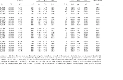
are listed in column (i) of Table 1. Columns (ii) and (iii) report the span and scope of the tick-by-tick data for each rate. For 11 currency pairs I use a decade of tick-by-tick bid and offer rates starting at midnight on December 31 st., 2003. Continuous data is not available for the other currency pairs in 2004 – 2007 so I use tick-by-tick rates starting after midnight on December 31st 2007, when continuous data becomes available. The data samples for all the currency pairs end at midnight on December 31 st., 2013. As column (iii) shows,
the time series for each currency pair contains tens of millions of data points. Each series contains a date and time stamp, where time is recorded to the nearest 1/100 of a second, and a bid and offer rate. Unlike standard time series, the time between observations is irregular, ranging from a few minutes to a hundredth of a second.
Gain Capital aggregates data from more than 20 banks and brokerages in the Forex market to construct
the bid and offer rates for each currency pair. To gauge how accurately these data represent rates across the Forex market, Gain provides a comparison of the mid-point between its bid and ask rates with the mid-point for the best tradable bid and ask rates aggregated from 150 market participants by an independent firm, Interactive Data Corporation GTIS. These comparisons (available on line at http://www.forex.com/pricing-comparison.html) show very small differences between the two mid-point series in current data, typically less
than one pip.12
As a further check on the accuracy of the Gain data, I compared the mid-points from the tick-by-tick data with the 4:00 pm Fix benchmarks on each trading day in the sample. Recall that the Fix benchmarks are computed as the mid point of the median bid and ask rates across multiple transactions in one minute
window that starts 30 seconds before 4:00 pm. For comparison I computed an analogous mid-point from the median of the bid and ask rate data on every trading day covered by each currency pair. Differences
12In the Forex market a “pip” typically refers to the fourth decimal place in a spot rate, i.e., the di
between this mid-point and the Fix represent the tracking error of the Gain data relative to the rates used to determine the Fix.13
Table 1 reports the percentiles of the tracking-error distribution, measured in basis points relative to the Fix benchmark, for each of the currency pairs I study. Since the behavior of spot rates around the Fix on the
last trading day in each month have been subject to particular scrutiny by the financial press, I separate the tracking errors on these days from the errors on other trading days and report percentiles for both the intra-and end-of-month distributions. Table 1 shows that the tracking errors in the Gain data are typically very small. The center panel of the table shows that the vast majority of intra-month tracking errors are within
±2 basis points. This represents a high level of accuracy. For perspective, column (xii) reports the average
spread between the bid and ask rates for each currency pair between 3:00 and 5:00 pm GMT. Clearly, most of the tracking-error distributions lie within these average spreads. The distributions for the end-of-month tracking errors are a little more dispersed: the 5’th. and 95’th. percentiles reported in columns (ix) and (xi) are larger (in absolute value) than their counterparts in the intra-month distributions (see columns (v) and (vii)). That said, the vast majority of the end-of-month tracking errors are still very small, both in absolute
terms and relative to the average spreads.
Table 1 also reports the number of trading days used to compute the tracking-error distributions in columns (iv) and (viii). In my analysis below I only use the Gain tick-by-tick data on days where the time-stamps for each bid and ask rate can be exactly matched to GMT. Unfortunately, this is not always possible.
There are days where the bid and ask rates with time-stamps that should correspond to 4:00 pm are clearly far from the Fix, so there must be a recording error in the Gain archive. I do not use any of the Gain data on these days. The different trading day numbers reported in columns (iv) and (viii) reflect the effects of this data verification process as well as differences in the data spans across currency pairs.
In summary, the statistics in Table1 show that once the accuracy of the time-stamps in the Gain data
has been verified, the tick-by-tick rates around the 4:00 pm very closely match the rates used in computing the actual Fix. Importantly, the tracking errors documented here are much smaller in magnitude than the changes in rates we will examine in the periods before and after the 4:00 pm, so the Gain data provides an accurate measure of how forex rates behave across the market around the Fix.
2.2
Statistical Methods
The statistical methods I use below are chosen to highlight how the behavior of spot rates around the end-of-month Fixes differ from their behavior around intra-month Fixes, and other times. To accommodate the fact
that the time series for intraday rates are irregularly spaced (i.e., the time between consecutive observations differs from observation to observation), I use a set of “observation windows” that define market events in clock time around the 4:00 pm. The set of observation windows are shown in Table 2. They range in duration from 11 hours starting at 7:00 am and ending at 6:00 pm, to just two minutes between 3:59 and 4:01 pm. For each window on every trading day with reliable Gain data I compute statistics that summarize
the behavior of the mid-point rate (i.e., the average of the bid and offer rates) within the window. These statistics include the first and last rates, the maximum and minimum rates.
13All calculations are undertaken using Matlab.
Table 1: Data Characteristics
Intra Month Trading Days End-of-Month Trading Days
FX Rate Data Span Prices Number Tracking Error Distribution Number Tracking Error Distribution Average Percentiles (basis points) Percentiles (basis points) Spread
(millions) 5% 50% 95% 5% 50% 95% (basis points)
(i) (ii) (iii) (iv) (v) (vi) (vii) (viii) (ix) (x) (xi) (xii)
A: EUR/USD 2004-13 55.370 2420 -1.113 0.055 1.209 117 -1.232 0.109 1.771 1.708
CHF/USD 2004-13 51.966 2258 -1.510 0.060 1.761 106 -2.462 0.058 2.345 3.477
JPY/USD 2004-13 38.931 2204 -1.268 0.140 1.790 104 -3.241 0.207 2.608 2.771
USD/GBP 2004-13 60.859 2421 -1.087 0.083 1.200 116 -1.258 0.051 2.566 2.285
B: CHF/EUR 2004-13 37.858 2373 -1.144 0.000 1.145 116 -2.135 0.000 1.243 2.160
JPY/EUR 2004-13 78.813 2421 -1.538 0.021 1.542 117 -4.939 0.090 2.822 2.622
NOK/EUR 2008-13 15.780 1291 -1.710 0.008 2.015 62 -2.624 0.252 3.829 4.449
NZD/EUR 2008-13 56.633 1414 -2.211 0.079 2.381 68 -2.927 0.284 3.844 7.018
SEK/EUR 2008-13 17.424 1288 -1.643 -0.010 1.551 59 -2.336 -0.089 1.980 3.584
C: AUS/GBP 2008-13 68.169 1476 -1.209 0.225 1.730 69 -2.695 0.544 4.016 4.773
CAD/GBP 2008-13 57.455 1478 -1.180 0.293 1.777 71 -1.676 0.371 2.578 4.841
CHF/GBP 2004-13 83.686 2417 -1.476 0.087 1.634 116 -3.412 0.020 2.013 4.152
EUR/GBP 2004-13 41.643 2339 -1.651 0.114 2.176 115 -2.302 0.157 2.523 3.208
JPY/GBP 2004-13 88.578 2418 -1.564 0.020 1.582 116 -2.612 0.137 2.378 4.090
NZD/GBP 2008-13 58.216 1409 -2.197 0.089 2.350 67 -2.529 0.397 5.046 9.738
D: AUS/USD 2004-13 49.016 2398 -1.601 0.144 2.283 116 -2.373 -0.117 2.053 3.171
CAD/USD 2004-13 36.163 2404 -1.461 0.138 1.864 116 -1.909 0.256 2.821 3.576
DKK/USD 2008-13 66.719 1305 -0.696 0.081 0.825 59 -0.779 0.115 0.996 1.244
NOK/USD 2008-13 55.350 1306 -1.696 0.071 2.152 62 -3.983 0.602 3.999 4.738
SEK/USD 2008-13 58.296 1297 -1.811 0.053 1.792 59 -2.783 0.101 2.067 4.048
SGD/USD 2008-13 10.567 1200 -1.440 0.000 1.517 61 -1.980 0.168 1.982 3.671
Notes: Columns (i) - (iii) show the data span and the number of quotes (in millions) for each of the currency pairs in the data set. Columns (iv) and (viii) report the number of intra-month and end-of-month trading days for which there are intraday quotes, respectively. Quote errors on each day are defined as the difference between the mid-point of the average bid and ask quotes computed over a 30 second window centered on 4:00 pm and the Fix benchmark. Quote errors are expressed in basis points. Columns (v) - (vii) and (ix) - (xi) show the 5th., 50th. and 95th. percentiles of the quote error distribution computed on all intra-month and end-of-month trading days. Column (xii) reports the average spread (in basis points) between the bid and ask quotes between 3:00 and 5:00 pm.
Table 2: Observation Windows
Window Start Time End Time Duration
(i) 7:00 am 6:00 pm 11 hrs
(ii) 3:00 pm 5:00 pm 2 hrs
(iii) 3:30 pm 4:30 pm 1 hr
(iv) 3:45 pm 4:15 pm 30 mins
(v) 3:50 pm 4:10 pm 20 mins
(vi) 3:55 pm 4:05 pm 10 mins
(vii) 3:56 pm 4:04 pm 8 mins
(viii) 3:57 pm 4:03 pm 6 mins
(ix) 3:58 pm 4:02 pm 4 mins
(x) 3:59 pm 4:01 pm 2 mins
I also use the Gain data to constructed empirical distributions for intraday spot rate dynamics away from the Fix. To build these distributions I pick a random starting time between 7:00 am and 6:00 pm on any day from the span of the intraday time series for a specific rate. I then use this time as the starting time for
nine observation windows that range in duration from two hours to two minutes. These randomly selected windows correspond to windows (ii) to (x) in Table 2. If any of the randomly selected windows cover the Fix or the release of U.S. macro data at 8:30 am EST, I discard the starting time. If not, I compute and record the same series of statistics for each of the nine windows (again using mid-point rates). This process is repeated 10,000 times to build up the empirical distribution of the rate statistics away from the Fix. It
is important to exclude observation windows that cover the scheduled releases of U.S. macro data when constructing these empirical distributions because the releases are often accompanied by large rate changes. These empirical distributions provide a benchmark to quantify differences between the behavior of spot rates around the Fix and other periods of normal trading activity.
In the next 4 sections I examine the behavior of rates around the Fix. To begin I take a macro perspective.
Fix benchmarks are routinely used to identify the daily spot rates from which the time series of exchange rates over months, years and decades are constructed, yet they are derived from spot rates contained in a very narrow window of daily trading activity. Section 3 examines the implications of this limitation. Next, in Section 4, I describe the behavior of spot rates under normal trading conditions. This analysis establishes
empirical metrics that are used when I study the behavior of rates immediately before and after 4:00 pm in Sections 5 and 6, respectively.
3
Daily Trading Ranges and the Fix
The forex market operates continuously, without any set opening or closing times, but in reality most trading is heavily concentrated on weekdays between approximately 7:00 am and 6:00 pm GMT. In contrast, the
spot rates used to compute the Fix come from a tiny window of daily trading activity: 30 seconds either side of 4:00 pm. Consequently, each day’s Fix provides limited information on the rates at which currencies trade throughout the trading day. Here I examine the implications of this limitation when studying the behavior of spot rates over days, months and longer horizons.
Figure 2: Major Currency Fixes with Daily Trading Range
05 06 07 08 09 10 11 12 13
1.15 1.2 1.25 1.3 1.35 1.4 1.45 1.5 1.55 1.6
EUR/USD
05 06 07 08 09 10 11 12 13
0.7 0.8 0.9 1 1.1 1.2 1.3 1.4
CHF/USD
05 06 07 08 09 10 11 12 13
75 80 85 90 95 100 105 110 115 120 125
JPY/USD
05 06 07 08 09 10 11 12 13
1.4 1.5 1.6 1.7 1.8 1.9 2 2.1
USD/GBP
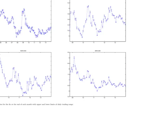
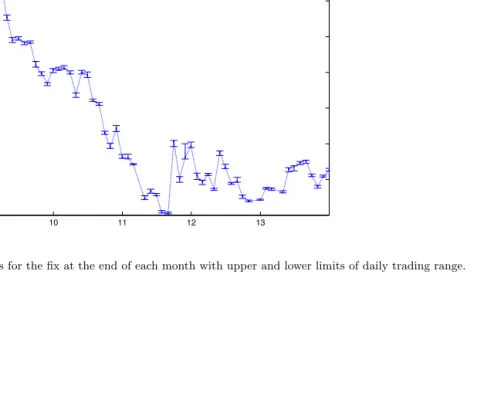
Notes: Time series for the Fix at the end of each month with upper and lower limits of daily trading range.
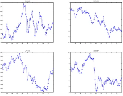
The Fix benchmarks are routinely used as daily rates when constructing time series for spot exchange rates over days, months or years. Figure 2 plots monthly time series for the spot rates of the four major currency pairs using the end-of-month Fixes between the end of 2003 and 2013. The plots also show the upper and lower limits for (mid-point) rates between 7:00 am and 6:00 pm GMT on the last trading day
of each month. As these plots clearly indicate, the low frequency variations in the level of each spot rate (between one and five years in duration) are orders of magnitude larger than the daily rate ranges. Thus the low frequency time series characteristics of spot rates appear robust to the use of the Fix to identify the end-of month rates. One way to visualize this is to imagine alternative plots where the end-of-month rate is pinned down by a randomly chosen point within the daily trading range. The plots would undoubtedly
features as the plots in Figure 2. In sum, therefore, the use of the Fix to identify the daily spot rate does not materially affect how we view the evolution of exchange-ratelevels over long horizons.
Figure 3: Daily Trading Ranges around the Fix
EUR/USD
05 06 07 08 09 10 11 12 13
−200 −150
−100 −50
0 50 100 150 200 250 300
CHF/USD
05 06 07 08 09 10 11 12 13
−250 −200 −150 −100
−50
0 50 100 150 200
JPY/USD
05 06 07 08 09 10 11 12 13
−200 −150 −100 −50 0 50 100 150 200
USD/GBP
05 06 07 08 09 10 11 12 13
−150 −100 −50
0 50 100 150 200 250
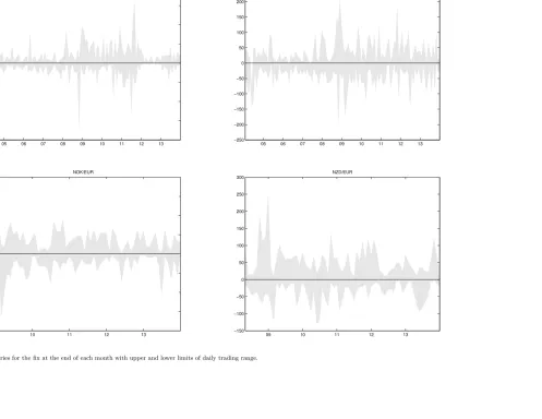
Notes: Each panel plots the daily price range at the end of each month as a band around the Fix price in basis points. The upper and lower edges of the band are equal to (lnPh
t−lnP
f
t)10000 and−(lnP f
t−lnPtl)10000, respectively; whereP f
t is the Fix price,Pthis the maximum price andPtlis the minimum price between 7:00 am and 6:00 pm
GMT on dayt.
While daily spot rate ranges are small compared to the long-term swings in the level of rates, they are
nevertheless sizable. Figure 3 illustrates this point for the major currency pairs. Here I plot the daily range at the end of each month as a band around the Fix in basis points. Thus the upper and lower edges of the band are equal to 10000(lnSmax
t lnS
f ix
t ) and 10000(lnS f ix
t lnStmin), respectively; whereS f ix t is the
Fix benchmark, Smax
t is the maximum rate andStmin is the minimum rate between 7:00 am and 6:00 pm
on day t. As the plots clearly show, the ranges are sometimes as large as a couple of hundred basis points (particularly during the 2008-2009 financial crisis), and are often at least a hundred basis points. Notice, also, that the bands are rarely symmetric around zero because the Fix is often far from the center of the daily range; a point I shall return to below. As in Figure 2, these plots are representative of the bands for the other currency pairs shown in the Appendix.
One way to judge the economic significance of the daily spot rate ranges is to compare them against prior changes in the Fix over different horizons. For this purpose, I compute the range-to-change ratio
Rn = (lnStmax lnStmin)/|lnS f ix
t lnS
f ix
t−n| at the end of each month for horizons n of one month, one
quarter and one year. Rn is just the ratio of the daily range (in percent) on dayt to the absolute value of
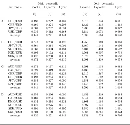
the percentage change in the Fix from dayt nto dayt. Table 3 reports the 50th. and 90th. percentiles of the empirical distributions forRn at three horizons for all the currency pairs. As the table shows, for all
the currency pairs both the 50’th. and 90’th. percentiles fall as the horizon rises from one month to one year. This is indicative of the leftward shift in theRn distributions asnrises, which is not at all surprising.
What is surprising are the size of ratios. To understand why, suppose an investor initiated a position at the Fix at the end of last month that was closed out at today’s Fix, a month later, with a 1 percent return. If
Rn= 0.5 today, and the investor had the discretion to close out the position at any time between 7:00 am
and 6:00 pm, he could have potentially achieved a return as large as 1.5 percent or as small as 0.5 percent, depending on where today’s Fix was set relative to the daily range. In this sense the median values forRn
imply that monthly and quarterly returns computed from Fix benchmarks are “typically” rather imprecise measures of the return an investor might have received had they initiated and/or closed their positions away from the Fix on the same days. Moreover, on at least ten percent of the days covered by the sample, returns
computed from the Fix could have been very imprecise. As the right hand columns of Table 3 show, the 90’th. percentiles of theRn distributions are in many cases above one. In these instances it is possible that
the return an investor received on a position initiated at the Fix but closed away from the Fix would have
adifferent sign from one closed at the Fix.
The results in Table 3 make clear that forex returns computed over macro-relevant horizons are sensitive to the time of day that positions are initiated and closed. Unless investors are known to only execute their forex trades at the Fix, conventional measures of returns on forex positions that use the Fix as the daily exchange rate arepotentially very imprecise measures of the returns actual investors received from positions initiated and closed on the same days. Of course the exact level of imprecision depends on far the rates
received by the investor on their transactions to initiate and close the position differ from the Fix. These calculations require trading data on individual investors. In contrast, most of the research literature on the carry trade, forward premium puzzle, and international portfolio diversification implicitly assumes that the ability to trade away from the Fix has no material affect on Forex returns over macro horizons. At the very least, the results in Table 3 cast some doubt on this assumption.
The results in Table 3 also provide a perspective on why so many forex trades are executed at the Fix. When an investor sells a foreign currency denominated security (e.g. a stock or bond) held in a custodian account, the proceeds from the sale are used to purchases domestic currency that is credited to the investor’s account. The results in the Table 3 show that the (domestic currency) return the investor ultimately receives could be materially affected if the custodian has discretion to choose the rate for the forex trade within the
range on the day the security is sold. Indeed the choice of rate for such forex trades has been the subject of litigation between institutional investors (mutual and pension funds) and custodial banks.14 One way to
avoid such litigation is to eliminate discretion over the rate used in custodial forex trades by specifying that they are executed at the Fix. This arrangement increases the level of transparency in custodial trades for institutional investors and also produces a flow of orders into the forex market to execute trades at the Fix.
Table 3: Range-to-Change Ratios
Rn= (lnSmax
t lnSmint )/|lnS f ix
t lnS
f ix t−n|
50th. percentile 90th. percentile
horizonsn 1 month 1 quarter 1 year 1 month 1 quarter 1 year
(i) (ii) (iii) (iv) (v) (vi)
A: EUR/USD 0.430 0.222 0.107 2.016 1.646 0.611
CHF/USD 0.460 0.224 0.203 2.527 1.518 1.418
JPY/USD 0.369 0.207 0.084 2.230 1.420 0.372
USD/GBP 0.536 0.312 0.168 5.184 2.071 0.989
Average 0.449 0.241 0.141 2.989 1.664 0.848
B: CHF/EUR 0.547 0.288 0.123 4.258 1.969 0.366
JPY/EUR 0.367 0.214 0.094 3.460 1.144 0.596
NOK/EUR 0.560 0.303 0.131 2.104 1.403 0.502
NZD/EUR 0.405 0.192 0.114 1.561 0.907 0.738
SEK/EUR 0.478 0.290 0.111 2.075 1.772 0.688
Average 0.472 0.257 0.115 2.691 1.439 0.578
C: AUD/GBP 0.372 0.177 0.116 2.991 1.115 0.982
CAD/GBP 0.529 0.419 0.235 3.433 1.777 1.164
CHF/GBP 0.451 0.278 0.123 2.616 1.567 0.558
GBP/EUR 0.493 0.264 0.172 3.896 1.832 0.980
JPY/GBP 0.383 0.227 0.096 1.181 0.903 0.959
NZD/GBP 0.416 0.238 0.142 1.443 1.912 1.390
Average 0.441 0.267 0.147 2.593 1.518 1.005
D: AUD/USD 0.355 0.236 0.096 1.457 1.319 0.385
CAD/USD 0.469 0.284 0.136 2.544 1.364 0.694
DKK/USD 0.432 0.214 0.121 1.861 1.163 0.534
NOK/USD 0.470 0.275 0.215 2.597 1.141 1.570
SEK/USD 0.491 0.304 0.195 2.286 4.565 1.161
SGD/USD 0.304 0.190 0.099 2.084 0.861 0.373
Average 0.420 0.251 0.144 2.138 1.735 0.786
Notes: The table reports percentiles of the empiricalRndistributions for each of the exchange rates listed on the left. Empirical distributions are constructed from the values forRncomputed at the end of each month for which reliable intraday rate data is available.
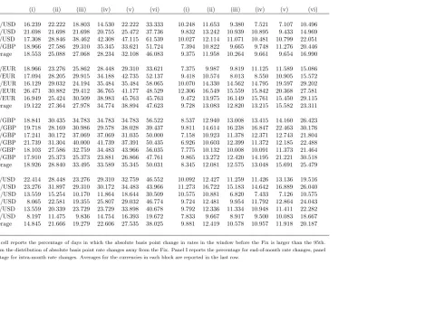
Table 4 reports statistical results that compliment the visual evidence in Figure 3 on the relation between the daily spot rate range and the Fix at the end of each month. The table provides information on the intraday rate ranges between 7:00 am and 6:00 pm, 3:00 and 5:00 pm, and between 3:30 and 4:30 pm on every day for which there is reliable data for each currency pair. Columns (i) and (ii) report the 50th. and 90th. percentiles of the empirical distribution for the range expressed in basis points; i.e., 10000(ln(Smax) ln(Smin)) where
Smax and Smin are the highest and lowest (mid-point) rates within the range. The tail probabilities in
columns (iii) and (iv) compare the Fix to the range on each day. Specifically, column (iii) reports the
fraction of days on which the ratio (Sf ix Smin)/(Smax Smin) is either below 0.1 or above 0.9, while
column (iv) reports fraction on which the ratio is either below 0.05 or above 0.95.
An inspection of the statistics in Table 4 reveals several noteworthy features. First, there is remarkable similarity in the empirical range distributions across currency pairs. Column (i) shows that typical spot rate
ranges (represented by the 50th. percentiles) from 7:00 am to 6:00 pm are between 70 and 80 basis points, fall to around 30 points between 3:00 and 5:00 pm, and are on average a little above 20 points between 3:30 and 4:30 pm. The 90th. percentiles for the range distributions are also very similar across most currency pairs, and are roughly twice the size of the 50th percentiles. Four currency pairs prove exceptions to this pattern: Distributions for the CHF/EUR and SGD/USD are shifted more to the left, while those for the
NOK/USD and SEK/USD are shifted more to the right.
The second noteworthy feature concerns the effect of time on the range distributions. As one would expect, the distributions shift leftward and become more compact as the ranges are computed over shorter time windows. Notice, however, that the statistics in panel III are based from just one hour of trading activity whereas those in panel I come from 11 hours. If the sequence of intraday rates followed a random
walk with a constant variance, the percentiles in panel I should be p11'0.33 times their counterparts in panel III. The table shows that this is approximately the case. This is surprising because the statistics in panel I encompass periods during which macro data are routinely released, whereas those in panel III come from the hour of trading around the Fix where releases do not occur. The factors affecting rates around the
Fix appear comparable in their effects on the range of rates as the release of macro data. This is one piece of evidence documenting the atypical behavior of spot rates around the Fix.
The third feature concerns the tail probabilities reported in columns (iii) and (iv). As the table clearly shows, the Fix appears close to the edges of the price ranges far more often that we would expect if it were merely a randomly chosen point from the range. For a perspective, consider the position of an investor who
is committed to undertaking a forex trade on a particular day and must decide whether to execute the trade via the submission of a standard (market or limit) order at a time close to 4:00 pm, or via the submission of a fill-at-fix order. The tail probabilities in panels II and III imply that the investor faces more rate uncertainty in orders filled at the Fix than from standard trades executed at a random time around the fix.
In summary, the results above show that the Fix provides limited information about the rates used in
the execution forex trades on any particular day. The Fix is computed as an average of rates in a narrow one-minute window that cannot adequately represent the fully range of spot rates at which trades take place over the trading day. As a consequence, investors initiating and closing positions away from the Fix are quite likely to achieve returns over days, weeks and longer, that differ significantly from those computed over the same horizons using the Fix. Furthermore, the Fix should not be viewed as representing a randomly
Table 4: Trading Ranges and the Fix
I: 7:00 am -6:00 pm GMT II: 3:00-5:00 pm GMT III: 3:30-4:30 pm GMT
Range Distribution Tail Probabilities Range Distribution Tail Probabilities Range Distribution Tail Probabilities
50% 90% 20% 10% 50% 90% 20% 10% 50% 90% 20% 10%
(i) (ii) (iii) (iv) (i) (ii) (iii) (iv) (i) (ii) (iii) (iv)
A: Majors EUR/USD 73.049 133.130 0.304 0.210 32.923 64.408 0.408 0.270 22.312 44.659 0.392 0.251
CHF/USD 79.157 142.709 0.321 0.216 35.972 68.733 0.396 0.253 24.611 48.101 0.359 0.232
JPY/USD 66.341 120.889 0.304 0.197 29.651 59.880 0.373 0.243 20.715 39.984 0.346 0.234
USD/GBP 68.880 129.649 0.279 0.177 29.767 59.391 0.357 0.228 20.757 42.069 0.338 0.213
Average 71.857 131.594 0.302 0.200 32.078 63.103 0.384 0.248 22.099 43.703 0.359 0.232
B: EUR CHF/EUR 32.996 90.981 0.340 0.222 15.306 41.911 0.334 0.208 11.164 30.955 0.315 0.184
JPY/EUR 79.185 163.978 0.299 0.192 35.100 74.383 0.363 0.235 24.073 52.200 0.364 0.222
NOK/EUR 61.523 121.154 0.272 0.163 28.879 55.579 0.277 0.167 20.754 41.480 0.246 0.156
NZD/EUR 82.317 151.633 0.298 0.204 38.680 76.462 0.340 0.201 28.393 57.282 0.309 0.194
SEK/EUR 65.110 129.011 0.260 0.153 29.969 57.276 0.283 0.174 22.076 41.735 0.250 0.166
Average 64.226 131.352 0.294 0.187 29.587 61.122 0.319 0.197 21.292 44.730 0.297 0.185
C: GBP AUS/GBP 79.906 155.525 0.294 0.202 36.362 74.123 0.361 0.230 26.683 57.060 0.338 0.205
CAD/GBP 82.238 153.473 0.288 0.176 38.710 76.689 0.315 0.203 27.846 56.795 0.305 0.212
CHF/GBP 66.053 133.963 0.286 0.190 28.722 59.177 0.357 0.220 20.951 43.033 0.333 0.209
EUR/GBP 57.296 112.261 0.248 0.154 23.686 46.904 0.327 0.192 17.273 34.743 0.302 0.173
JPY/GBP 81.113 165.301 0.293 0.177 34.818 75.997 0.347 0.232 24.917 54.822 0.325 0.212
NZD/GBP 86.413 161.864 0.297 0.187 41.723 82.508 0.335 0.202 30.252 63.275 0.298 0.197
Average 75.503 147.064 0.284 0.181 34.003 69.233 0.340 0.213 24.654 51.621 0.317 0.201
D: USD AUS/USD 78.218 161.009 0.329 0.218 37.792 81.713 0.368 0.227 27.054 56.649 0.330 0.196
CAD/USD 74.574 137.799 0.284 0.181 35.149 70.505 0.329 0.202 24.847 48.947 0.303 0.186
DKK/USD 80.139 146.297 0.304 0.216 37.026 70.223 0.410 0.267 25.234 49.993 0.398 0.263
NOK/USD 105.594 197.482 0.311 0.198 50.165 94.826 0.347 0.220 35.640 67.861 0.330 0.202
SEK/USD 110.334 209.301 0.299 0.192 51.952 98.312 0.350 0.213 36.553 70.112 0.325 0.203
SGD/USD 36.736 67.820 0.313 0.185 16.850 31.507 0.344 0.225 11.549 23.386 0.313 0.189
Average 80.932 153.285 0.307 0.198 38.156 74.515 0.358 0.226 26.813 52.825 0.333 0.206
Notes: Columns (i) and (ii) report the 50th. and 90th. percentiles from the empirical distribution of the trading range (identified in the header of each panel) expressed in basis points; i.e., (ln(Smax
)−ln(S
min
))10000 whereSmax
andSmin
are the highest and lowest mid-point rates within the range. Column (iii) reports the fraction of days in the sample that the ratio (Sf ix
−S
min )/(Smax
−S
min
) is either below 0.1 or above 0.9. Column (iv) reports the fraction of the days when the ratio is either below 0.05 or above 0.95.
4
Spot Rate Dynamics Away from the Fix
In this section I examine the behavior of intraday spot rate dynamics away from the Fix. Table 5 reports statistics for the distribution of spot rate changes over horizons of five, fifteen, and thirty minutes. These statistics are computed from an empirical distribution of 10000 observations chosen at random times (away from the Fix) from the time series of intraday (mid-point) rates,{St}, for each currency pair (as described in
Section 2.2). Columns (iii) - (vii) report statistics for the distribution of changes in the log rates expressed in basis points per minute, i.e.,∆ hs
t ⌘(ln(St+h) ln(St))⇤10000/h for horizonsh={5,15,60} minutes.
Columns (viii) and (ix) report the first-order autocorrelation in∆ hst (i.e. corr(∆hst+h,∆hst)) and the
p-value for the null of a zero autocorrelation, respectively. Column (x) reports the Kolmogorov-Smirnov (KS) test for the null that the two conditional distributionsf(∆hs
t+h|∆hst>0) andf(∆hst+h|∆hst0)
are the same.15
The p-value for the test is shown in column (xi).
As Table 5 shows, the rate-change distributions have several common characteristics across all the cur-rency pairs. First, the dispersion in the rate-change distributions decline as the horizon rises. Columns (iii) and (iv) show that the absolute values for the 5th. and 95th. percentiles of the distributions fall as the horizon rise from five to 30 minutes. The change in dispersion is also reflected by the standard deviations
shown in column (v), which fall as the horizon rises. Second, all the rate-change distributions are strongly leptokurtic. As column (vii) shows, the kurtosis statistics across all the currency pairs are large; much larger than the value of three for the implied by the normal distribution. These statistics indicate that atypically large changes in rates occur quite frequently away from the Fix and scheduled macro news releases.
The third feature concerns temporal dependence between rate changes. Column (viii) shows that rate changes display some small degree of autocorrelation. Across currency pairs, the autocorrelation is generally negative. This fact accounts for the declining dispersion of the rate-change distributions as the horizon rises, noted above. Although small in (absolute) value, the statistics in column (ix) indi-cate that many of the estimated autocorrelation coefficients are statistical signifiant at standard levels.
There is also evidence of temporal dependence from the KS tests reported in column (ix). Under the null of temporal independence, future changes in rates should not depend on the sign of past changes, i.e., f(∆hs
t+h|∆hst > 0) = f(∆hst+h|∆hst 0). As column (x) shows, this null can easily be rejected at
standard levels of significance for most currency pairs and horizonsh.
15
Two versions of the KS test can be found in the statistics literature. The one-sample KS test is a nonparametric test of the null hypothesis that the population cdf of the data is equal to the hypothesized cdf. The two-sample KS test is a nonparametric hypothesis test of the null that the data in two samples are from the same continuous distribution. Here I compute the two-sample KS test which uses the maximum absolute difference between the cdfs of the distributions of the two data samples. The test statistic is computed asD=maxx
⇣
|Fˆ1(x)−Fˆ2(x)| ⌘
where ˆF1(x) is the proportion of the first data sample less than
or equal tox, and ˆF2(x) is the proportion of the second data sample less than or equal tox.The KS test and its asymptotic