Applicative structure in vector space models

Applicative structure in vector space models

M´arton Makrai D´avid Nemeskey

HAS Computer and Automation Research Institute H-1111 Kende u 13-17, Budapest

{makrai,ndavid,kornai}@sztaki.hu

Andr´as Kornai

Abstract

We introduce a new 50-dimensional em-bedding obtained by spectral clustering of a graph describing the conceptual struc-ture of the lexicon. We use the embedding directly to investigate sets of antonymic pairs, and indirectly to argue that func-tion applicafunc-tion in CVSMs requires not just vectors but two transformations (cor-responding to subject and object) as well.

1 Introduction

Commutativity is a fundamental property of vec-tor space models. As soon as we encodekingby

~_{k,queenby~q,malebym~, andfemalebyf}~_{, if we}

expect~k´~q “ m~ ´f~, as suggested in Mikolov et al. (2013), we will, by commutativity, also ex-pect~k´m~ “ ~q´f~‘ruler, gender unspecified’. When the meaning decomposition involves func-tion applicafunc-tion, commutativity no longer makes sense: considerVictoriaas~qmEnglandandVictor as~kmItaly. If the function application operatorm

is simply another vector to be added to the rep-resentation, the same logic would yield that Italy is the male counterpart of female England. To make matters worse, performing the same oper-ations onAlbert,~kmEngland andElena, ~qmItaly would yield that Italy is the female counterpart of male England.

Section 2 offers a method to treat antonymy in continuous vector space models (CVSMs). Sec-tion 3 describes a new embedding, 4lang, obtained by spectral clustering from the definitional frame-work of the Longman Dictionary of Contempo-rary English (LDOCE, see Chapter 13 of McArtur 1998), and Section 4 shows how to solve the prob-lem outlined above by treating mandnnot as a vectors but as transformations.

2 Diagnostic properties of additive decomposition

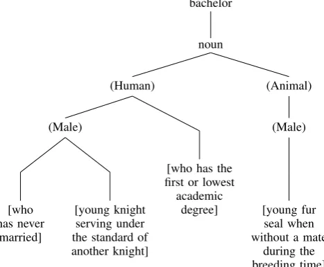
The standard model of lexical decomposition (Katz and Fodor, 1963) divides lexical meaning in a systematic component, given by a tree of (gener-ally binary) features, and an accidental component they call thedistinguisher. Figure 1 gives an ex-ample.

bachelor

noun

(Animal)

(Male)

[young fur seal when without a mate

during the breeding time] (Human)

[who has the first or lowest academic

degree] (Male)

[young knight serving under the standard of another knight] [who

has never married]

Figure 1: Decomposition of lexical items to fea-tures (Katz and Fodor, 1963)

This representation has several advantages: for example bachelor3 ‘holder of a BA or BSc de-gree’ neatly escapes beingmaleby definition. We tested which putative semantic features likeGEN

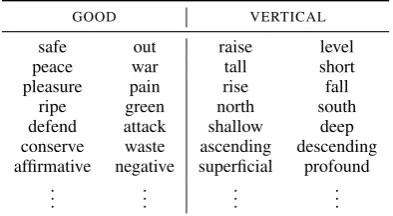
-DERare captured by CVSMs. We assume that the difference between two vectors, for antonyms, dis-tills the actual property which is the opposite in each member of a pair of antonyms. So, for ex-ample, for a set of male and female words, such asxking, queeny,xactor, actressy, etc., the differ-ence between words in each pair should represent the idea of gender. To test the hypothesis, we

GOOD VERTICAL

safe out raise level

peace war tall short

pleasure pain rise fall

ripe green north south

defend attack shallow deep conserve waste ascending descending affirmative negative superficial profound

..

. ... ... ...

Table 1: Word pairs associated to features GOOD

andVERTICAL

sociated antonymic word pairs from the WordNet (Miller, 1995) to 26 classes e.g.END/BEGINNING,

GOOD/BAD, . . . , see Table 1 and Table 3 for

ex-amples. The intuition to be tested is that the first member of a pair relates to the second one in the same way among all pairs associated to the same feature. For k pairs ~xi, ~yi we are looking for a

common vector~asuch that

~

xi´~yi “~a (1)

Given the noise in the embedding, it would be naive in the extreme to assume that (1) can be a strict identity. Rather, our interest is with the best

~awhich minimizes the error

Err “ ÿ

i

||x~i´~yi´~a||2 (2)

As is well known, E will be minimal when~ais chosen as the arithmetic mean of the vectorsx~i´

~

yi. The question is simply the following: is the

minimalEmany better than what we could expect

from a bunch of randomx~iand~yi?

Since the sets are of different sizes, we took 100 random pairings of the words appearing on either sides of the pairs to estimate the error distribution, computing the minima of

Errrand“ ÿ

i

||x~i1´~yi1´~a||2 (3)

For each distribution, we computed the mean and the variance ofErrrand, and checked whether

the error of the correct pairing,Erris at least 2 or 3σs away from the mean.

Table 2 summarizes our results for three embed-dings: the original and the scaled HLBL (Mnih and Hinton, 2009) and SENNA (Collobert et al., 2011). The first two columns give the number of pairs considered for a feature and the name of the

PRIMARY ANGULAR

leading following square round preparation resolution sharp flat

precede follow curved straight intermediate terminal curly straight antecedent subsequent angular rounded precede succeed sharpen soften question answer angularity roundness

..

. ... ... ...

Table 3: Features that fail the test

feature. For each of the three embeddings, we re-port the errorErrof the unpermuted arrangement, the meanmand varianceσ of the errors obtained under random permutations, and the ratio

r“ |m´Err|

σ .

Horizontal lines divide the features to three groups: for the upper group, r ě 3 for at least two of the three embeddings, and for the middle groupr ě2for at least two.

For the features above the first line we conclude that the antonymic relations are well captured by the embeddings, and for the features below the second line we assume, conservatively, that they are not. (In fact, looking at the first column of Ta-ble 2 suggests that the lack of significance at the bottom rows may be due primarily to the fact that WordNet has more antonym pairs for the features that performed well on this test than for those fea-tures that performed badly, but we didn’t want to start creating antonym pairs manually.) For exam-ple, the putative sets in Table 3 does not meet the criterion and gets rejected.

3 Embedding based on conceptual representation

The 4lang embedding is created in a manner that is notably different from the others. Our input is a graph whose nodes are concepts, with edges run-ning fromAtoB iffBis used in the definition of

A. The base vectors are obtained by the spectral clustering method pioneered by (Ng et al., 2001): the incidence matrix of the conceptual network is replaced by an affinity matrix whoseij-th element is formed by computing the cosine distance of the

ith andjth row of the original matrix, and the first few (in our case, 100) eigenvectors are used as a basis.

# feature HLBL original HLBL scaled SENNA

pairs name Err m σ r Err m σ r Err m σ r

156 good 1.92 2.29 0.032 11.6 4.15 4.94 0.0635 12.5 50.2 81.1 1.35 22.9 42 vertical 1.77 2.62 0.0617 13.8 3.82 5.63 0.168 10.8 37.3 81.2 2.78 15.8 49 in 1.94 2.62 0.0805 8.56 4.17 5.64 0.191 7.68 40.6 82.9 2.46 17.2

32 many 1.56 2.46 0.0809 11.2 3.36 5.3 0.176 11 43.8 76.9 3.01 11

65 active 1.87 2.27 0.0613 6.55 4.02 4.9 0.125 6.99 50.2 84.4 2.43 14.1 48 same 2.23 2.62 0.0684 5.63 4.82 5.64 0.14 5.84 49.1 80.8 2.85 11.1 28 end 1.68 2.49 0.124 6.52 3.62 5.34 0.321 5.36 34.7 76.7 4.53 9.25 32 sophis 2.34 2.76 0.105 4.01 5.05 5.93 0.187 4.72 43.4 78.3 2.9 12 36 time 1.97 2.41 0.0929 4.66 4.26 5.2 0.179 5.26 51.4 82.9 3.06 10.3 20 progress 1.34 1.71 0.0852 4.28 2.9 3.72 0.152 5.39 47.1 78.4 4.67 6.7

34 yes 2.3 2.7 0.0998 4.03 4.96 5.82 0.24 3.6 59.4 86.8 3.36 8.17

23 whole 1.96 2.19 0.0718 3.2 4.23 4.71 0.179 2.66 52.8 80.3 3.18 8.65 18 mental 1.86 2.14 0.0783 3.54 4.02 4.6 0.155 3.76 51.9 73.9 3.52 6.26 14 gender 1.27 1.68 0.126 3.2 2.74 3.66 0.261 3.5 19.8 57.4 5.88 6.38

12 color 1.2 1.59 0.104 3.7 2.59 3.47 0.236 3.69 46.1 70 5.91 4.04

17 strong 1.41 1.69 0.0948 2.92 3.05 3.63 0.235 2.48 49.5 74.9 3.34 7.59 16 know 1.79 2.07 0.0983 2.88 3.86 4.52 0.224 2.94 47.6 74.2 4.29 6.21 12 front 1.48 1.95 0.17 2.74 3.19 4.21 0.401 2.54 37.1 63.7 5.09 5.23 22 size 2.13 2.69 0.266 2.11 4.6 5.86 0.62 2.04 45.9 73.2 4.39 6.21 10 distance 1.6 1.76 0.0748 2.06 3.45 3.77 0.172 1.85 47.2 73.3 4.67 5.58 10 real 1.45 1.61 0.092 1.78 3.11 3.51 0.182 2.19 44.2 64.2 5.52 3.63 14 primary 2.22 2.43 0.154 1.36 4.78 5.26 0.357 1.35 59.4 80.9 4.3 5 8 single 1.57 1.82 0.19 1.32 3.38 3.83 0.32 1.4 40.3 70.7 6.48 4.69 8 sound 1.65 1.8 0.109 1.36 3.57 3.88 0.228 1.37 46.2 62.7 6.17 2.67 7 hard 1.46 1.58 0.129 0.931 3.15 3.41 0.306 0.861 42.5 60.4 8.21 2.18 10 angular 2.34 2.45 0.203 0.501 5.05 5.22 0.395 0.432 46.3 60 6.18 2.2

Table 2: Error of approximating real antonymic pairs (Err), mean and standard deviation (m, σ) of error with 100 random pairings, and the ratior“ |Err_σ´m|for different features and embeddings

element wi corresponds to a base vector bi. For

the vocabulary of the whole dictionary, we sim-ply take the Longman definition of any word w, strip out the stopwords (we use a small list of 19 elements taken from the top of the frequency dis-tribution), and formVpwqas the sum of thebifor

thewis that appeared in the definition ofw(with

multiplicity).

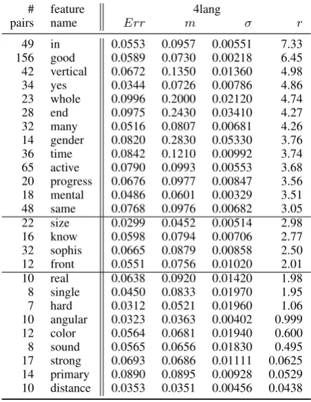
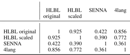
We performed the same computations based on this embedding as in Section 2: the results are pre-sented in Table 4. Judgment columns under the four three embeddings in the previous section and 4lang are highly correlated, see table 5.

Unsurprisingly, the strongest correlation is be-tween the original and the scaled HLBL results. Both the original and the scaled HLBL correlate notably better with 4lang than with SENNA, mak-ing the latter the odd one out.

4 Applicativity

So far we have seen that a dictionary-based em-bedding, when used for a purely semantic task, the analysis of antonyms, does about as well as the more standard embeddings based on cooccurrence data. Clearly, a CVSM could be obtained by the same procedure from any machine-readable

dic-# feature 4lang

pairs name Err m σ r

49 in 0.0553 0.0957 0.00551 7.33

156 good 0.0589 0.0730 0.00218 6.45 42 vertical 0.0672 0.1350 0.01360 4.98 34 yes 0.0344 0.0726 0.00786 4.86 23 whole 0.0996 0.2000 0.02120 4.74 28 end 0.0975 0.2430 0.03410 4.27 32 many 0.0516 0.0807 0.00681 4.26 14 gender 0.0820 0.2830 0.05330 3.76 36 time 0.0842 0.1210 0.00992 3.74 65 active 0.0790 0.0993 0.00553 3.68 20 progress 0.0676 0.0977 0.00847 3.56 18 mental 0.0486 0.0601 0.00329 3.51 48 same 0.0768 0.0976 0.00682 3.05 22 size 0.0299 0.0452 0.00514 2.98 16 know 0.0598 0.0794 0.00706 2.77 32 sophis 0.0665 0.0879 0.00858 2.50 12 front 0.0551 0.0756 0.01020 2.01 10 real 0.0638 0.0920 0.01420 1.98 8 single 0.0450 0.0833 0.01970 1.95 7 hard 0.0312 0.0521 0.01960 1.06 10 angular 0.0323 0.0363 0.00402 0.999 12 color 0.0564 0.0681 0.01940 0.600 8 sound 0.0565 0.0656 0.01830 0.495 17 strong 0.0693 0.0686 0.01111 0.0625 14 primary 0.0890 0.0895 0.00928 0.0529 10 distance 0.0353 0.0351 0.00456 0.0438

HLBL HLBL SENNA 4lang original scaled

HLBL original 1 0.925 0.422 0.856

HLBL scaled 0.925 1 0.390 0.772

SENNA 0.422 0.390 1 0.361

4lang 0.856 0.772 0.361 1

Table 5: Correlations between judgments based on different embeddings

tionary. Using LDOCE is computationally advan-tageous in that the core vocabulary is guaranteed to be very small, but finding the eigenvectors for an 80k by 80k sparse matrix would also be within CPU reach. The main advantage of starting with a conceptual graph lies elsewhere, in the possibility of investigating the function application issue we started out with.

The 4lang conceptual representation relies on a small number of basic elements, most of which correspond to what are called unary predicates in logic. We have argued elsewhere (Kornai, 2012) that meaning of linguistic expressions can be for-malized using predicates with at most two argu-ments (there are no ditransitive or higher arity predicates on the semantic side). The x and y

slots of binary elements such as x has yor x kill y, (Kornai and Makrai 2013) receive distinct la-bels called NOM andACC in case grammar (Fill-more, 1977); 1 and 2 in relational grammar (Perl-mutter, 1983); orAGENT andPATIENTin linking

theory (Ostler, 1979). The label names themselves are irrelevant, what matters is that these elements are not part of the lexicon the same way as the words are, but rather constitute transformations of the vector space.

Here we will use the binary predicate x has y to reformulate the puzzle we started out with, an-alyzing queen of England, king of Italy etc. in a compositional (additive) manner, but escaping the commutativity problem. For the sake of concrete-ness we use the traditional assumption that it is the king who possesses the realm and not the other way around, but what follows would apply just as well if the roles were reversed. What we are inter-ested in is the asymmetry of expressions like Al-bert has EnglandorElena has Italy, in contrast to largely symmetric predicates. Albert marries Vic-toria will be true if and only ifVictoria marries Albertis true, but fromJames has a martiniit does not follow that?A martini has James.

While the fundamental approach of CVSM is quite correct in assuming that nouns (unaries) and verbs (binaries) can be mapped on the same space, we need two transformations T1 and T2 to regulate the linking of arguments. A form like James kills has James as agent, so we com-puteV(James)`T1V(kill), whilekills Jamesis ob-tained as V(James)`T2V(kill). The same two transforms can distinguish agent and patient rel-atives as in the man that killed James versusthe man that James killed.

Such forms are compositional, and in languages that have overt case markers, even ‘surface com-positional’ (Hausser, 1984). All input and outputs are treated as vectors in the same space where the atomic lexical entries get mapped, but the applica-tive paradox we started out with goes away. As long as the transformsT1(n) andT2(m) take dif-ferent values onkill, has,or any other binary, the meanings are kept separate.

Acknowledgments

Makrai did the work on antonym set testing, Nemeskey built the embedding, Kornai advised. We would like to thank Zs´ofia Tardos (BUTE) and the anonymous reviewers for useful comments. Work supported by OTKA grant #82333.

References

R. Collobert, J. Weston, L. Bottou, M. Karlen, K. Kavukcuoglu, and P. Kuksa. 2011. Natural lan-guage processing (almost) from scratch. Journal of Machine Learning Research (JMLR).

Charles Fillmore. 1977. The case for case reopened. In P. Cole and J.M. Sadock, editors, Grammatical Relations, pages 59–82. Academic Press.

Roland Hausser. 1984. Surface compositional gram-mar. Wilhelm Fink Verlag, M¨unchen.

J. Katz and Jerry A. Fodor. 1963. The structure of a semantic theory.Language, 39:170–210.

Andr´as Kornai and M´arton Makrai. 2013. A 4lang fogalmi sz´ot´ar [the 4lang concept dictionary]. In A. Tan´acs and V. Vincze, editors, IX. Magyar Sz´amit´og´epes Nyelv´eszeti Konferencia [Ninth Con-ference on Hungarian Computational Linguistics], pages 62–70.

Tom McArthur. 1998. Living Words: Language, Lex-icography, and the Knowledge Revolution. Exeter Language and Lexicography Series. University of Exeter Press.

Tomas Mikolov, Kai Chen, Greg Corrado, and Jeffrey Dean. to appear. Efficient estimation of word repre-sentations in vector space. In Y. Bengio, , and Y. Le-Cun, editors,Proc. ICLR 2013.

George A. Miller. 1995. Wordnet: a lexical database for english. Communications of the ACM, 38(11):39–41.

Andriy Mnih and Geoffrey E Hinton. 2009. A scalable hierarchical distributed language model. Advances in neural information processing systems, 21:1081– 1088.

Andrew Y. Ng, Michael I. Jordan, and Yair Weiss. 2001. On spectral clustering: Analysis and an algo-rithm. InAdvances in neural information processing systems, pages 849–856. MIT Press.

Nicholas Ostler. 1979. Case-Linking: a Theory of Case and Verb Diathesis Applied to Classical San-skrit. PhD thesis, MIT.