Predicting the Rainfall of Ghana using the Grey Prediction Model GM(1,1) and the Grey Verhulst Model

© 2019, IRJET | Impact Factor value: 7.34 | ISO 9001:2008 Certified Journal

| Page 1362

Predicting the Rainfall of Ghana using the Grey Prediction Model

GM(1,1) and the Grey Verhulst Model

Peter Derickx Davis

_{, Grace Amankwah}

_{, Professor Qiquan Fang}

1,3

_{School of Science, Zhejiang University of Science and Technology}

Hangzhou, Zhejiang Province, China

2

_{School of Information and Electrical Engineering, Zhejiang University of Science and Technology, Hangzhou,}

Zhejiang Province, China

---***---

and the environment largely depends on the impact of rainfall patterns and climate change. The study of rainfall pattern is critical as it has great influx in the resolution of the several environment phenomenon of water resource managements, with diverse implications on agriculture, sustainability and development. Data analysis and forecasting are key components resolved to understudy these phenomena with several development interventions to mitigate the negative impact on the society and economy. The main objective of this study is to predict the rainfall variability of Ghana from 2017 - 2024. The Grey Prediction Model GM (1,1) and the Grey Verhulst Model (GVM) is used to forecast the rainfall patterns for these years. The analysis of the prediction results is illustrated for future implications and development interventions.

Keywords: GM(1,1), Grey Verhulst Model, Rainfall

1.

Rain water over the past years has served as an essential part of our lives, varying form global development to an individual daily use [1]. The use of rain water is seen variably in the areas of agricultural production, power generation, industrial water supply, sanitation and disease prevention [2]. In Ghana, the agricultural sector offers a great source of employment for the 300,000-350,000 workers employed each year by the government. Agriculture employs a greater number of unskilled workers and more extensively serves a s source of income for more than 70 percent of the rural population, as well as a greater part of the country’s poorest households [3]. However, this sector largely depends solely on rainfall to survive. There have been recent studies on the effect of rainfall on agricultural production [4], migration [5], poverty [6], health and education [7], food security [8] among others. It is realised that rainfall pattern has a great influence on various sectors of a nation’s economy and livelihood. However, extreme rainfall conditions such as floods and droughts have overwhelming direct and indirect effects [9]. Direct effect like agriculture and infrastructure is primarily obvious, whereas indirect effects such as the reluctance to invest in a risk-prone area has serious

economic implications. Droughts and floods can subsequently damage economic growth. Recent studies reveal that a 1 percent influx in affected areas has the tendency to slow down a country’s Gross Domestic Product by 2.7 percent per year, and 1 percent increase in areas experiencing floods reduce Gross Domestic Product by 1.8 percent [10]. Many rural households sort to the use of informal approaches for managing weather related risks [11]. Nevertheless, depending on informal assurance to manage weather variations from others in the same city or region may not be effective and unreliable since rainfall patters and variability can be difficult to predict [12].

The study therefore seeks to analyse the rainfall variability of Ghana and predict the annual variability for the successful years using the GM(1,1) and the Grey Verhaulst Model (GVM) to support decision-making, planning and designing in the respective fields of agriculture and hydrology.

1.1 Significance of the research

The research paper has the following objectives:

 to analyse the rainfall variability of Ghana from 2009 – 2016 and to establish a set of standard models for forecasting the prediction of the rainfall variability from 2017 – 2024 using the GM(1,1) Model and the Grey Verhaulst model.

 using the forecasting models for prediction will not only help in identifying the rainfall variability for the following years but help improve decision making towards development and planning in the water and agriculture sectors. This will help add to existing knowledge on rainfall variability in Ghana.

2. Literature Review

2.1 The Evolution of Grey System Theory

© 2019, IRJET | Impact Factor value: 7.34 | ISO 9001:2008 Certified Journal

| Page 1363

understanding between objects and events enriching the overall progress of science and technology. Many issues identified in the prehistoric times have been adequately solved and new systems developed in modern sciences, leading to a clearer apprehension of the laws governing object evolutions. System theories, information theories and cybernetics came to play in the 1940s, among others such as synergics, dissipative structures, bifurcations and catastrophe appearing in 1960 to 1970. In the 20th century there is seemingly an increase in the discovery and application of system sciences. For instance; the introduction of Fuzzy Mathematics by L. A. Zadeh in 1960, Grey system Analysis by Julong Deng in 1970, among others. All these and many system theories have contributed to the knowledge application of system sciences [20].

2.2 Uncertain Systems

The primary physiognomies of uncertain systems are their scantiness and incompleteness in their evidence. Uncertain systems commonly exist due to the subtleties of many system evolutions, biological limitations of the human sensing organs, and the constraints of relevant economic conditions and the disposal or availability of technology. There are mainly three system theories known to be the most research methods widely used for the investigation of uncertain systems, but they are seemingly different with respect to their characteristics.

2.2.1 Fuzzy Mathematics

The theory of Fuzzy Mathematics highlights on the study of problems with perceptive uncertainty, where the research objects possess the characteristic of clear intension and unclear extension. Take for instance; “a young man”. This poses a fuzzy concept because a very person can identify the characteristics of a young man. However, a man young does not portray a clear intension because it is not easy to determine the range at which one can classified which is young or not. This kind of phenomenon of cognitive uncertainty with clear intension and unclear extension is handled in fuzzy mathematics by experience and the so-called membership function [20].

2.2.2 Probability and Statistics

Probability and Statistics also analyses the issues of uncertainty with importance on revealing the historical statistical laws. They however probe for the occurrence of possible outcome of the stochastic uncertainties. This theory deals with the available starting points of large samples, which are essential in satisfying a certain typical form of distribution.

2.2.3 Grey System

Grey systems theory captures uncertainty problems of small samples and poor information that are challenging

for probability and fuzzy mathematics to handle. One of its characteristics is construct models with small amounts of data. The difference between fuzzy mathematics and grey systems theory is that fuzzy mathematics emphasizes on the examination of such objects with unknown boundaries. For example, by the year of 2050, China will control its total population within the range of 1.5 to 1.6 billion people. This range from 1.5 billion to 1.6 billion is a grey concept. Its extension is definite and clear. However, if one inquires further regarding exactly which specific number within the said range it will be, then he will not be able to obtain any meaningful and definite answer.

2.3 The application range of grey system theory

Grey system theory has been widely used, not only successfully applied in engineering control, economic management, social systems, ecosystems, etc., but also in complex and varied agricultural systems, such as in water conservancy, meteorology, biological control, agricultural machinery. Decision-making, agricultural planning, and agricultural economics have also made gratifying achievements. Grey system theory has shown a wide range of application prospects in the fields of management, decision-making, strategy, forecasting, futurology, and life sciences.

Grey system seeks the law of its development and change by collecting and sorting the original data. This is because the phenomena manifested by the objective system are complicated, but their development has its own objective logic and is the system. Coordination and unification of the overall functions, therefore, how to find the inherent development law through the scattered data series is particularly important. The grey system theory holds that all grey sequences can exhibit their original laws by weakening their randomness by some kind of generation, that is, establishing a system reaction model through grey data sequences, and predicting the possible change state of the system through the model.

2.4 The GM (1,1) Model of Grey System Analysis and the Verhaulst Model

2.4.1 The GM(1,1) Model

© 2019, IRJET | Impact Factor value: 7.34 | ISO 9001:2008 Certified Journal

| Page 1364

Partial and inaccurate data is the rudimentary nature of uncertainty system. In the literature [23], the author gave an extensive discussion of the characteristics of uncertainty system and the role of the uncertainty model in the research of uncertainty systems [24]. It evidently revealed that pursuing the thorough model in the case of inadequate information and inaccurate data was impossible. In fact, Lao Zi had this very brilliant exposition two thousand years ago: invisible, inaudible, no touch, the three cannot be explained clearly.

The founder of fuzzy mathematics Professor Zadeh’s (L.A. Zadeh) incompatibility theory also vividly specified that when the density of a system is growing, the ability to make an accurate and significant account of a system’s characteristics declines, until it attains a threshold value that, if it exceeds the value, the precision and significance would become two mutually exclusive characteristics [25]. Incompatibility principle proves that pursuing fine, one-sidedly will result in low feasibility and significance of recognition results. Refined model is an ineffective means to deal with complex matters. A large number of practical systems which people faced have the characteristics of incomplete information, of which many famous scholars have clear conclusions [26]. It is prevalent in the real-world uncertainty systems that involves small data and inaccurate information and it offers rich resources for further studies in the grey system theory.

In the last thirty years, the research of Model GM(1,1) has been very active due to the practical needs, and new research results are continuously emerging. There have been many studies with the objective of focusing on how to further heighten the model and to expand the simulated and predictive results. Buffer operator [27] surfaced in 1991 and it had attracted much attention in recent years [28]. It is essentially a system for processing raw data, rather than a method to advance the degree of accuracy of prediction and simulation model. During the period that the researchers are collecting the raw data, the system is subject to interference from external shocks, then the data must be distorted and be difficult to reflect the operation of the system behaviour. In this instance, people have the option to choose or construct a suitable buffer operator conferring to the qualitative analysis of the results to disregard the influence of the distort data sequence and retain the true nature of the data [29].

2.4.2 The Grey Verhulst Model

The Verhulst Model was introduced by a German Biologist, Pierre Franos Verhulst. The model was to define the increasing process like the “S” curve which has a saturation region or sigmoid process [30]. The Grey Verhulst Model is a time series prediction model which is established by using a first order differential equation [31]. This model is often used to predict

human populations, biological growth, reproduction, and economic life span of consumable products, among others [21].

3. Methodology 3. 1 The GM(1,1) Model

The basic and commonly used model of Grey model is

GM(1,1), which is known as the first-order differential model with only one input variable. This model is used to implement the short-term forecasting operation which has no strict hypothesis for distribution of original data series.

3.3.1 Model definition

Given the sequence of data ( )_{, we simulate the}

sequence by using the GM(1,1) model. Let

( ) _[ ( )_{( )} ( )_{( )} ( )_{( )] (3.1)}

where ( )_{(𝑘) ≥ 0}

Taking ( ) _{we compute the Accumulation Generation of} ( )_{: that is}

(1) _{[( )} (1)_{( ) ⋯} (1)_{( )] (3.2)}

where (1)_{(𝑘) ∑}𝑘 ( )_(𝑖)

𝑖=1  𝑘 ⋯ .

Then ( )_{(𝑘) + 𝑎} (1)_{(𝑘) 𝑏 (3.3)}

is referred to as the original form of model GM(1,1), and actually it is a different equation.

By using the adjacent neighbours of (1)_{, we obtain the}

neighbour means sequence;

(1) _[ (1)_{( )} (1)_{( )} (1)_{( ) (3.4)}

Let ( ) (1) _and (1) _{be the same above.}

[

(1) ( )

(1)_{( )}

(1)_{( ) ]}

[ ( )_{( )}( )

( )

( )_{( )]}

(3.5)

By using the least square estimate, we obtain the sequence of parameters 𝑎̂ [𝑎 𝑏] as follows;

𝑎̂ ( ) 1 _*𝑎

𝑏+

We establish the model

+ 𝑎

1 _{𝑏 (3.6)}

© 2019, IRJET | Impact Factor value: 7.34 | ISO 9001:2008 Certified Journal

| Page 1365

The simulated values are defined by;

̂1 _{[ ̂}1_{( ) ̂}1_{( ) ̂}1_{( )] (3.8)}

By using the formula;

̂ (𝑘) (1) _̂1_{(𝑘) ̂}1_{(𝑘) (𝑘 ) (3.9)}

3.2 The Grey Verhulst Model

For an initial time sequence, of raw data ( )_, (1) _the

sequence of accumulation generation of ( )_and (1) _the

adjacent neighbour mean of generation (1)_{. The}

GM(1,1) power model becomes;

( )_{(𝑘) + 𝑎} (1)_{(𝑘) 𝑏[} (1)_{(𝑘)] (3.10)}

[

(1)( ) ( (1)( )) (1)_{( ) (} (1)_{( ))}

(1)_{( ) (} (1)_{( )) ]}

[ ( )_{( )}( )

( )

( )_{( )]}

(3.11)

The equation (3.10) can be obtained by using the least square method, of the parametric sequence 𝑎̂ [𝑎 𝑏] . The equation becomes then;

𝑎̂ ( ) 1

The solution for the Verhulst whitenization equation is;

( )

+ 𝑎

(1) _𝑏( (1)_{) (3.12)}

and the time response sequence for the model is

̂1_{(𝑘 + )} ( )( )

( )_{( ) [} ( )_{( )]} (3.13)

3.3 Error Checking

The study involves certain error checks that were used to measure the performance rate and to demonstrate the level of accuracy of the two proposed forecasting models. The four accuracy evaluation standards for the study includes; the Relative Percentage Error (RPE), the Root Mean Squared Error (RMSE), the Mean average Percentage Error (MAPE) and the Precision Rate (PR).

3.3.1 The Relative Percentage Error (RPE)

The RPE depicts the variance or difference between the actual values and the simulated values. The purpose of this method is to measure the amount of error as a percentage of the actual values. The RPE formula is represented as follows [32]:

[ (𝑘)] ( )(𝑘) ̂_{( )(𝑘)}(𝑘) (3.14)

3.3.2 The Root Mean Squared Error (RMSE)

The RMSE is a method for estimating the forecasting accuracy that deals with the sample standard deviation

(SD) of the difference between the actual values and the predicted values.

√∑ [ ( )(𝑘) ̂ (𝑘)] _(3.15)

3.3.3 The Mean Average Percentage Error (MAPE) MAPE is an accuracy formula widely applied in forecasting. It’s also referred to as the Average Relative Percentage Error (ARPE) which denotes the average relative size between the original data values and the predicted values. Relatively, it is the mean of the RPE

[21].

(1∑𝑘=1 ( )(𝑘) ̂_{( )(𝑘)}(𝑘)) 00 (3.16)

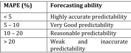
The forecasting model is interpreted to be highly accurate when the MAPE value is less than 5. It is considered to be a good precision model when the MAPE is between 5 and 10. When the MAPE is more than 20, the model is said to be inaccurate [33].

Table 1: Evaluation for Model Precision MAPE (%) Forecasting ability

< 5 Highly accurate predictability

5 – 10 Very Good predictability

10 – 20 Reasonable predictability

> 20 Weak and inaccurate

predictability

Interpretation of the MAPE results

The Precision Rate (P) is used to determine the level of closeness of the statement of the forecasted values and the actual values. The value of (P) is however defined as;

(3.17)

The developing coefficient a of the grey model is also considered as a measure to determine the forecasting capacity of a particular grey model. The value interpretation is illustrated in Table 2 [21].

Table 2: Forecasting Capacity of Model Range of

Development Coefficient (a)

Interpretation Forecasting Capacity of Model

𝑎 0. Simulation

accuracy above 98%

For medium

and long-term forecasting

0. 𝑎

0. Simulation accuracy above 90%

© 2019, IRJET | Impact Factor value: 7.34 | ISO 9001:2008 Certified Journal

| Page 1366

0. Simulation accuracy above 80%

Carefully used for short-term forecasting

0. 𝑎 Simulation

accuracy lower than 70%

Not suitable for forecasting

𝑎 . Simulation

accuracy lower than 50%

Not suitable for forecasting

4. Forecasting the Rainfall Variability in Ghana 4.1 Selection of Sample Area

The sample area for the study is the rainfall variability of Ghana which is located in the West Coast of Africa and shares boundaries with Togo, Burkina Faso and La Cote d’Ivoire, The study area has a total land area of 238,535km2 _{and lies geographically between longitude}

1.20°E and 3.25°W and latitude 4.50°N and 11.18°N [34]. Ghana has 10 administrative regions with a total population of 30.42 million with a population density of 121 people per square kilometre [35]. The country’s climatic condition is defined as tropical with two seasons; namely the cold or wet season and the hot or dry season. Due to the African Monsoon winds, Ghana experiences rainy seasons during summer. Rainy seasons however, lasts from May to September in the North, April to October in the centre of the country and from April to November in the South. The rainy season is nevertheless shorter along the coastal areas and usually lasts from the months of April to June, and some few rains from September and October [36].

Studies have proved that Ghana’s annual rainfall is high on inter‐annual and inter‐decadal timescales [37]. This explains why trying to identify long term trends have difficulties. Rainfall in Ghana have recorded high values since 1960. However, in the late 1970s and early 1980s, the level of rainfall reduced and showed a general decreasing trend from that period to 2008, with an average decreasing value of 2.3 mm monthly (2.4%) per decade. Multiple rainfall studies undertaken in Ghana only focused on designated stations or zones. For example, [38] focussed on Accra and Tamale, [39] concerted on Tamale, [40] concentrated on Wenchi, and [41] on northern Ghana. Nevertheless, few studies have taken Ghana as a whole. [42] researched on the trends in rainfall patterns in Ghana from 1960 to 2005, while [40] focused on the spatial pattern of rainfall in Ghana using RCMs modules. The current study however is aimed at predicting the rainfall variability over the whole of Ghana based on the following conditions;

 due to the uneven rainfall pattern of each year, the study considered a number of years in order to make good predictions,

 the rainfall data is that of the whole country (Ghana) but in different years, and

 these years are continuous, not intermittent, and there is no contingency, so the distribution of samples is reasonable.

4.2 Grey Model Establishment Steps

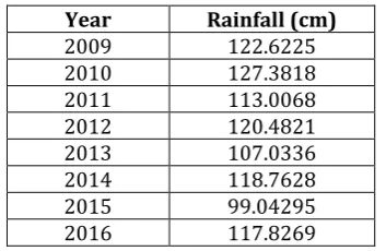
The rainfall data used for the study is the rainfall data of Ghana which covers the period from 2009 to 2016 and this is period where data was available. The data was ascertained from the Ghana Meteorological Agency (GMet). In this section the GM(1,1) and the Grey Verhulst Model are used for comparison. The rainfall data is used to prove the effectiveness and feasibilities of these models.

Table 3: Rainfall Data of Ghana from 2009 to 2016 Year Rainfall (cm)

2009 122.6225

2010 127.3818

2011 113.0068

2012 120.4821

2013 107.0336

2014 118.7628

2015 99.04295

2016 117.8269

Source: Ghana Meteorological Agency (GMet), 2016

4.2.1 The GM(1,1) Model

Given the sequence of our rainfall data ( )_{, we simulate}

the sequence by using the GM(1,1) model (𝑘) + 𝑎 (𝑘) 𝑏, where ( ) _{is our sequence of the raw data.}

( ) _[ ( )_{( )} ( )_{( )} ( )_{( )]}

( ) _[ ( )( ) ( )( ) ( )( ) ( )( ) ( )( )

( )_{( )} ( )_{( )} ( )_{( )} ]

This implies:

( ) _{[ . . .00 0.}

0 .0 . .0 . ]

Taking ( ) _{we compute the accumulation generation of} ( )_:

For (1)₌

[ (1)( ) (1)( ) (1)( ) (1)( ) (1)( ) (1)( )

(1)_{( )} (1)_{( )} ]

(1) _[ . 0.00 .0 . 0.

0 . 0 . . ]

© 2019, IRJET | Impact Factor value: 7.34 | ISO 9001:2008 Certified Journal

| Page 1367

It implies that ( ) 0. 0. ( ) 0. 0. ( ) 0. 0. ( ) 0. 0 0. ( ) 0. 0. ( ) 0. 0.

For 𝑘 , the condition of quasi-smoothness is satisfied.

We determine whether or not it complies with the law of quasi-exponentiality.

From 1_(𝑘) ( )𝑘

( )_{𝑘 1} it follows that 1( ) . , 1_{( ) 1.33,} 1_{( ) . ,} 1_{( ) . 0,} 1_{( ) 1.14,} 1_{( ) .}

So, for 𝑘 , 1_{(𝑘) [ . ] with 0. . Thus, the}

law of quasi-exponentiality is satisfied, therefore we can establish a GM(1,1) model for (1)_.

By using the adjacent neighbours of (1)_{, we obtain the}

`neighbour means sequence;

(1) _[ (1)_{( )} (1)_{( )} (1)_{( )} (1)_{( )} (1)_{( )} (1)_{( )} (1)_{( )}

(1) _{[ . 0 0 . 0 . 0}

.0 0 . 0 . . ]

[

(1)( )

(1)_{( )}

(1)_{( )}

(1)_{( )}

(1)_{( )}

(1)_{( )}

(1)_{( ) ]}

=

[

. 0 0 . 0 . 0 .0 0 . 0 . . ]

[ ( )_{( )}( )

( )

( )_{( )}

( )_{( )}

( )_{( )}

( )_{( )}

( )_{( )]}

[

. .00 0. 0 .0 . .0 . ]

By using the least square estimate, we obtain the sequence of parameters 𝑎̂ [𝑎 𝑏] as follows

𝑎̂ ( ) 1 _{* 0.0}

. +

We establish the model

1

+ 0.0 1 .

and its time response formula:

𝑎̂1_{(𝑘) [} ( )_{( )} 𝑏

𝑎] (𝑘 1)+

𝑏 𝑎

. . 1 (𝑘 1)_{+ 0 . 0}

Computing the simulated values

̂1 _[ ̂1( ) ̂1( ) ̂1( ) ̂1( ) ̂1( ) ̂1_{( ) ̂}1_{( ) ̂}1_{( )} ]

̂1 _{[ . . 0 . .}

. 0 0 . 0 . . 0 ]

Compute the simulated values of ( )_{by using}

̂ (𝑘) (1) _̂1_{(𝑘) ̂}1_{(𝑘) (𝑘 )}

̂( ) _[ . . .0 0 .

. 0 . 0. 0 . ]

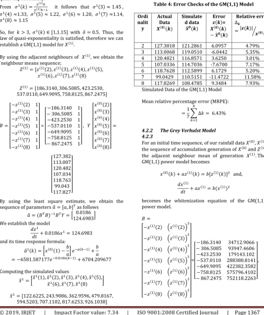
Table 4: Error Checks of the GM(1,1) Model Ordi

nalit y

Actual Data

( )_{( )}

Simulate d data

̂ ( )

Error ( )=

( )_{( )}

̂ ( )

Relative error

| ( )| ⁄( )_{( )}

2 127.3818 121.2861 6.0957 4.79%

3 113.0068 119.0510 -6.0442 5.35%

4 120.4821 116.8571 3.6250 3.01%

5 107.0336 114.7036 -7.6700 7.17%

6 118.7628 112.5899 6.1729 5.20%

7 99.0429 110.5151 -11.4722 11.58%

8 117.8269 108.4785 9.3484 7.93%

Simulated Data of the GM(1,1) Model

Mean relative percentage error (MRPE):

∑ 𝑘 𝑘=

.

4.2.2 The Grey Verhulst Model 4.2.3

For an initial time sequence, of our rainfall data ( )_, (1)

the sequence of accumulation generation of ( )_and (1)

the adjacent neighbour mean of generation (1)_{. The}

GM(1,1) power model becomes

( )_{(𝑘) + 𝑎} (1)_{(𝑘) 𝑏[} (1)_{(𝑘)] and,}

(1)

+ 𝑎 (1) 𝑏( (1))

becomes the whitenization equation of the GM(1,1) power model.

[

(1)( ) ( (1)_{( ))}

(1)_{( ) (} (1)_{( ))}

(1)_{( ) (} (1)_{( ))}

(1)_{( ) (} (1)_{( ))}

(1)_{( ) (} (1)_{( ))}

(1)_{( ) (} (1)_{( ))}

(1)_{( ) (} (1)_{( ))} ]

=

[

. 0 . 0

0 . 0 . 0

. 0 . 0

.0 0 0. . 0 . . . 0 . . ]

© 2019, IRJET | Impact Factor value: 7.34 | ISO 9001:2008 Certified Journal

| Page 1368

[ ( )_{( )}( )

( )

( )_{( )}

( )_{( )}

( )_{( )}

( )_{( )}

( )_{( )]}

[

. .00 0. 0 .0 . .0 . ]

By using the least square estimate, we obtain the sequence of parameters 𝑎̂ [𝑎 𝑏] as follows

𝑎̂ ( ) 1 _{* 0.}

0.000 +

Therefore, the whitenization equation is

(1)

0. (1) 0.000 0 ( (1))

By taking (1)₍₀₎ ( )_{( ) . we obtain the}

time response sequence

̂ (𝑘 + ) 𝑎 (1)(0)

𝑏 (1)_{(0) + [𝑎 𝑏} (1)_(0)] 𝑘 .

0.0 0 0. ( . )𝑘

Computing the simulated values

̂1 _[ ̂1( ) ̂1( ) ̂1( ) ̂1( ) ̂1( ) ̂1_{( ) ̂}1_{( ) ̂}1_{( )} ]

̂1 _{[ . . 0 . . 00}

.0 0 . . 0. ]

Compute the simulated values of ( )_{by using} ̂ (𝑘) (1) _̂1_{(𝑘) ̂}1_{(𝑘) (𝑘 )}

̂( ) _{[ . . . 0.}

. . .00 ]

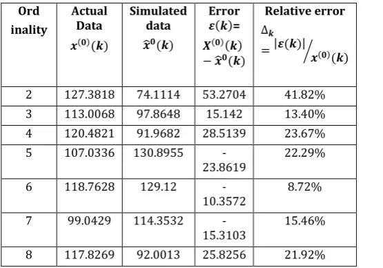
Table 5: Error Checks of the GVM Ord

inality

Actual Data ( )_{( )}

Simulated data

̂ ( )

Error

( )= ( )_{( )}

̂ ( )

Relative error

| ( )|

( )_{( )}

⁄

2 127.3818 74.1114 53.2704 41.82% 3 113.0068 97.8648 15.142 13.40% 4 120.4821 91.9682 28.5139 23.67% 5 107.0336 130.8955

-23.8619 22.29% 6 118.7628 129.12

-10.3572 8.72% 7 99.0429 114.3532

-15.3103 15.46% 8 117.8269 92.0013 25.8256 21.92%

From the table we obtain the mean relative error

∑ 𝑘

𝑘=

.0

Table 6: The Simulated Values and Error Values of the two Models

Tim e

Actual Data

( )_(𝑘)

GM(1,1) Model Grey Verhulst

Model (GVM)

Simulate d Value

̂ ( )

Relativ e Error (%)

Simulate d Value

̂ ( )

Relativ e Error (%)

201

0 127.382 121.2861 4.79 74.1114 41.82

201

1 113.007 119.0510 5.35 97.8648 13.40

201

2 120.482 116.8571 3.01 91.9682 23.67

201

3 107.034 114.7036 7.17 130.8955 22.29

201

4 118.763 112.5899 5.20 129.12 8.72

201

5 99.043 110.5151 11.58 114.3532 15.46

201

6 117.827 108.4785 7.93 92.0013 21.92

Comparison of the Simulated Data and Errors of the GM(1,1) and GVM

Figure 1: Actual Rainfall Data vs Simulated Values 0

20 40 60 80 100 120 140

2010 2011 2012 2013 2014 2015 2016

Rai

n

fal

l

Years

© 2019, IRJET | Impact Factor value: 7.34 | ISO 9001:2008 Certified Journal

| Page 1369

Index GM(1,1) GVM

RMSE 7.59 27.92

MAPE (%) 6.43 21.04

Precision rate

(%) 93.57 78.96

Forecasting

ability predictability Very good Inaccurate Weak and predictability

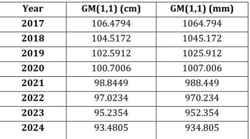
Table 8: Predicted Rainfall Values from 2017-2024 Year GM(1,1) (cm) GM(1,1) (mm)

2017 106.4794 1064.794

2018 104.5172 1045.172

2019 102.5912 1025.912

2020 100.7006 1007.006

2021 98.8449 988.449

2022 97.0234 970.234

2023 95.2354 952.354

2024 93.4805 934.805

Simulated Rainfall Data

From Table it is realised that the RMSE value of the GM(1,1) and the Grey Verhulst (GVM) are 7.59 and 27.92. Comparing the two models the GM(1,1) value is smaller. The MAPE values of the GM(1,1) and GVM are 6.34% and 21.04% respectively. The MAPE values reveals that the value of the GVM is the largest. The purpose of the MAPE is to measure the accuracy of the model used for the prediction. The GM(1,1) value has the smallest MAPE value and therefore has a high accurate prediction than the GVM model. The precision rate of the GM(1,1) is 93.57%. and that of the GVM records 78.96%. This reveals that the GM(1,1) has high accuracy than the GVM. Table 1 also reveals that the GM(1,1) model has a very good predictability because it has its MAPE between the values of 5 and 10. The GVM rather has a weak and inaccurate predictability because it has its MAPE to be greater than 20.

The developing coefficient (a) of grey models is used to assess the forecasting capacity of the proposed models. The coefficient (a) of the two models has been calculated and presented in Table 7. The development coefficients of both models are 0.0186 and 0.4745 for the GM(1,1) and GVM respectively. Referring to the table, the GM(1,1) is used for medium and long-term forecasting because it has a higher simulation accuracy. The GVM however, is suitable for short term prediction. The study considers predicting rainfall variables from 2017 to 2024 which is measured as a medium or long-term period. Based on the results from the two models, the accuracy of the

GM(1,1) model in forecasting the rainfall variability is higher than the Grey Verhulst Model. The GM(1,1) is inherently better because of its simplicity and also has a high forecasting precision.

5. Conclusions

From the study, it was revealed that the GM(1,1) predicted values were at a decreasing rate (Figure 1). According to Nkrumah F. et al (2014), the country’s rainfall pattern has had a decreasing trend from 1980 to 2008. The decreasing trend can however be seen in the rainfall pattern between 2009 and 2016 and this can also be seen in the forecasting values from 2017 to 2024 using the GM(1,1). This however reveals that the rainfall variability for the country has a decreasing pattern as such there must be development policies enacted to mitigate the impact of the decrease in rainfall. Rainfall has immense impact on various areas of the country’s economy such agriculture, power generation, vegetation, ecosystem among others therefore the decreasing tend of rainfall pattern must be given critical attention and great economic consideration.

The decrease in rainfall variability is a clear indication of global warming stemming from human activities such as urbanization, deforestation, overgrazing and people performing farming activities nearer to rivers and water bodies. Despite these challenges there is a decline in the rainfall pattern as revealed in the study. The prediction of rainfall is paramount because of its immense impact and benefits on the economy. In the case of agriculture, it is recommended that farmers and investors must be assisted by the GMet and agricultural extension officers to adjust to the rainfall patterns in order to prevent total crop failures. There is the need for intensive agricultural production to meet the increasing demand of population in the country. Changes in weather conditions such as droughts coupled with the decreasing rainfall patter will result in disaster in later years. Therefore, there is the need for social and environment interventions to create a sustainable agricultural system to protect and increase crop production for the increasing population. Farmers must also be informed and equipped to adopt to irrigation practices to relieve them of the total dependence on rainfall for farming.

© 2019, IRJET | Impact Factor value: 7.34 | ISO 9001:2008 Certified Journal

| Page 1370

and avenues made for solar equipment to be subsidized to encourage its patronage. Other sources of electricity include; the adoption of wind generated power, renewable energy, among others. This however can reduce the impact of the decrease rainfall pattern on the energy sector.

It is recommended that studies on rainfall be carried out extensively in order to gain adequate information on the country’s rainfall pattern and variability. Rainfall data is necessary to help inform policy makers on the best development decisions that will help the country’s agriculture, energy and water resource. This will also provide a platform for future investment in the rainfall variability of the country and will help innovations and developments in the institutions involved in the sector.

6. Acknowledgement

I express my deepest gratitude to Professor Qiquan Fang for his supervision and his immense support towards the completion of this paper.

REFERENCES

[1] UNWWD, “Water and Shared Responsibility. World Water Assessment Programme”, WWAP - UNESCO Division of Water Sciences, Paris Cedex 15, France, United Nations World Water Development Report 2, 2006.

[2] F. Y Logah1, E. Obuobie, D. Ofori, K. Kankam-Yeboah, “Analysis of Rainfall Variability in Ghana” (IJLREC) Volume 1, Issue 1: Page No.1, September-October 2013 [3] The World Bank Group, “Ghana: Agriculture Sector Policy Note, Transforming Agriculture for Economic Growth, Job Creation.” Agriculture Global Practice, West Africa (AFR01) Report. Page No. 19, June 2017.

[4] Levine, D., Yang, D., 2014. The Impact of Rainfall on Rice Output in Indonesia. NBER Working paper 20302.

[5] Mueller, V.A. and Osgood, D.E., 2009. Long-Term Consequences of Short-Term Precipitation Shocks:

Evidence from Brazilian Migrant Households.

Agricultural Economics. 40, 573-586.

[6] Barnett, B., Mahul, O., 2007. Weather index insurance for agriculture and rural areas in lower-income countries. American Journal of Agricultural Economics. 89, 1241-1247

[7] Maccini, S., Yang, D., 2009. Under the Weather, Health, Schooling, And Economic Consequences of Early-Life Rainfall. American Economic Review. 99, 1006-1026. [8] Birhanu, A., Zeller, M., 2009. Using Panel Data to Estimate the Effect of Rainfall Shocks on Smallholders Food Security and Vulnerability in Rural Ethiopia.

Research in Development Economics and Policy, Discussion Paper No. 2/2009.

[9] Pablo M., Antonio Y., 2015. “The Effect of Rainfall Variation on Agricultural Households: Evidence from Mexico”. International Conference of Agricultural Economist. Page No. 1, 2015.

[10] Brown, C., Meeks, R., Ghile, Y. et al. (2013). “Is Water Security Necessary? An Empirical Analysis of The Effects of Climate Hazards on National-Level Economic Growth”. Philosophical Transactions of the Royal Society A. 371: 20120416. DOI:10.1098/rsta.2012.04.16.

[11] Cheng, C.C., Chang, C.C., 2005. The Impact of Weather on Crop Yield Distribution in Taiwan: Some New Evidence from Panel Data Models and Implications for Crop Insurance. Agricultural Economics. 33, Issue Supplement s3, 503511.

[12] Gudiño, J., 2013. Los Microseguros: Un Instrumento Economico De Combate a La Pobreza. Ph.D. Thesis in Economics, Center For Economic Studies, El Colegio de Mexico.

[13] Stanturf, J. A., M. L. Warren, Susan Charnley, Sophia C. Polasky, Scott L. Goodrick, Frederick Armah, and Yaw Atuahene Nyako. "Ghana Climate Change Vulnerability and Adaptation Assessment." Washington: United States

Analyse spectrale des séries chronologiques des précipitations en Méditerranée occidentale", Agency for International Development (2011). Pg. 30-33

[14] Tabony, (1981): "A principal component and spectral analysis of European rainfall", Journal of Climatology, 1, pp 283-294.

[15] Djellouli and Daget (1989): "Le climat méditerranéen, change-t-il? Précipitations de quelques stations algériennes", Publications de l'AIC, vol. 2, pp 227-232.

[16] Maheras (1988): "Changes in precipitation conditions in the Western Mediterranean over the last century", Journal of Climatology, vol. 8, 179-189

[17] Maheras and Vafiaris (1990): " Publications de l'AIC, vol. 3, 421-429.

[18] Benito, Orellana, and Zurita (1994): "Análisis de la estabilidad temporal de los patrones de precipitación en la Península Ibérica", in PITA and AGUILAR (Ed): "Cambios y variaciones climáticas en España", Publicaciones de la Universidad de Sevilla, pp183 -193.

© 2019, IRJET | Impact Factor value: 7.34 | ISO 9001:2008 Certified Journal

| Page 1371

[20] Liu, Sifeng, and Yi Lin. "Introduction to Grey Systems Theory." Grey systems. Springer, Berlin, Heidelberg, 2010. pp 1.

[21] Deng J. L., Control problems of grey systems [J]. Systems & Control Letters, 1982, 1(5): 288-294

[22] Liu Sifeng, Lin Yi. Grey Systems: Theory and Applications[M]. Springer-Verlag, 2011.

[23] Liu Sifeng, Lin Yi. Grey Information: Theory and Practical Applications [M]. London: Springer-Verlag London Ltd, 2006.

[24] Liu Sifeng, Dang Yaoguo, Fang Zhigeng and Xie Naiming, Grey System Theory and Its Application [M] (5th Edition), Science Press, BeiJing, 2010.

[25] Lao-tzu. Tao Te Ching. Jiangsu Ancient Books Publisher, 2001.6

[26] Zadeh L A. Soft computing and Fuzzy Logic [J]. IEEE Software, 1994, 11(6): 48一56.

[27] Vallee, R. Book Reviews: Grey Information: Theory and Practical Applications[J]. Kybernetes, 2008, 37(1): 89.

[28] Andrew. A. M. Why the world is grey. Grey Systems: Theory and Application. 2011, Vol.1, No.2, pp 112-116

[29] Scarlat E., Delcea C. Complete analysis of bankruptcy syndrome using grey systems theory. Grey Systems: Theory and Application. 2011, Vol.1, No.1. pp.19-32

[30] Z. J. Guo, X. Q. Song, and J. Ye, Journal of the Eastern Asia Society for Transportation Studies, 6, 881 (2005).

[31] Ming, J., Fan, Z., Xie, Z., Jiang, Y., & Zuo, B. (2013). A Modified Grey Verhulst Model Method to Predict Ultraviolet Protection Performance of Aging B. Mori Silk Fabric. Fibers and Polymers, 14, 1179-1183.

[32] Hsu, L.-C. Applying the grey prediction model to the global integrated circuit industry. Technol. Forecast. Soc. Chang. 2003, 70, 563–574

[33] Xu, N., & Dang, Y. (2015). An Optimized Grey GM(2,1) Model and Forecasting of Highway Subgrade Settlement. pp 4.

[34] Logah, F.Y., Obuobie, E., Ofori, D.A., & Kankam-Yeboah, K. (2013). Analysis of Rainfall Variability in Ghana.

[35] Ghana Population. (07-12). Retrieved

2019-08-18, from

http://worldpopulationreview.com/countries/ghana/].

[36] Nkrumah, F., et al. (2014) Rainfall Variability over Ghana: Model versus Rain Gauge Observation. International Journal of Geosciences, 5, 673-683.

[37] McSweeney, C., Lizcano, G., New, M. and Lu, X. (2010) The UNDP Climate Change Country Profiles. http://journals.ametsoc.org/doi/abs/10.1175/2009BA MS2826.1

[38] Adiku, S.G.K., Mawunya, F.D., Jones, J.W. and Yangyouru, M. (2007) Can ENSO Help in Agricultural Decision Making in Ghana? In: Sivakumar, M. V. K. and Hansen, K., Eds., Climate Prediction and Agriculture, Springer, Berlin Heidelberg.

[39] Yengoh, G.T. (2010) Trends in Agriculturally-Relevant Rainfall Characteristics for Small-Scale Agriculture in Northern Ghana. Journal of Agricultural Science, 2, 3-16.

[40] Owusu, K. and Waylen, P.R. (2013) The Changing Rainy Season Climatology of Mid-Ghana. Theoretical and Applied Climatology, 112, 419-430.

[41] Friesen, J. (2002) Spatio-Temporal Patterns of Rainfall in Northern Ghana. Diploma Thesis, University of Bonn, Germany.