Coverage Performance in MIMO ZFBF Dense HetNets with Multiplexing and LOS/NLOS Path Loss Attenuation

Coverage Performance in MIMO-ZFBF Dense HetNets

with Multiplexing and LOS/NLOS Path-Loss Attenuation

Mohammad G. Khoshkholgh,

Memeber, IEEE, Keivan Navaie,

Senior Memeber, IEEE,

Kang G. Shin,

Life Fellow, IEEE, Victor C. M. Leung,

Fellow, IEEE

Abstract—The performance of multiple-input multiple-output (MIMO) multiplexing heterogenous cellular networks are often analyzed using a single-exponent path-loss model. Thus, the effect of the expected line-of-sight (LOS) propagation in densified settings is unaccounted for, leading to inaccurate performance evaluation and/or inefficient system design. This is due to the complexity of LOS/non-LOS models in the context of MIMO communications. We address this issue by developing an analytical framework based on stochastic geometry to evaluate the coverage performance. We focus on the zero-forcing beamforming where the maximum

signal-to-interference ratio is used for cell association. We analytically derive the coverage. We then investigate the cross-stream interference correlation, and develop two approximations of the coverage: Alzer Approximation (A-A) and Gamma Approximation (G-A). The former is often used in the single antenna and single-stream MIMO. We extend A-A to a MIMO multiplexing system and evaluate its utility. We show that the inverse interference is well-fitted by a Gamma random variable, where its parameters are directly related to the system parameters. The accuracy and robustness of G-A is higher than that of A-A. We observe that depending on the multiplexing gain, it is possible to attain the best coverage probability by proper densification.

Index Terms—Area spectral efficiency, coverage probability, densification, heterogenous cellular networks (HetNets), LOS/NLOS path-loss model, multiple-input multiple-output (MIMO), multiplexing, numerical complexity, Poisson Point Process (PPP), stochastic geometry, zero-forcing beamforming (ZFBF).

✦

1

INTRODUCTION

D

(Het-Nets) as well as air interface technology based on multiple-input multiple-output (MIMO) are viable ways to address the rapid and substantial growth of mobile data demand. In fact, these two technologies have been integral parts of the air interface technology in 5G and beyond [2], [3], thanks to a set of encouraging analytical results in [4], [5], [6], [7] demonstrating a nearly proportional growth of the area spectral efficiency (ASE) in HetNets by steadily increasing the number of BSs per unit area (densification) without deteriorating the coverage probability (scale invari-ance). These analytical results were developed by leveraging tools of stochastic geometry (e.g., [8], [9], [10], and validated with empirical studies, e.g., [11], [12].

• The paper received March 27, 2018, revised February 20, 2019 and May 17, 2019. The paper is accepted June 5, 2019. An earlier version of this work was presented in IEEE VTC-Fall, 2017, Toronto [1]. The corresponding author is V. C. M. Leung.

• M. G. Khoshkholgh (e-mail: [email protected]) is with the Department of Electrical and Computer Engineering, the University of British Columbia, Vancouver, BC, Canada V6T 1Z4; V. C. M. Leung is with the College of Computer Science and Software Engineering, Shenzhen University, Shenzhen 518060, China, and also with the Depart-ment of Electrical and Computer Engineering, The University of British Columbia, Vancouver, BC V6T 1Z4, Canada (e-mail:,[email protected]); K. Navaie (e-mail: [email protected]) is with the School of Computing and Communications, Lancaster University, Lancaster, United Kingdom LA1 4WA; K. G. Shin (e-mail: [email protected]) is with the Department of Electrical Engineering and Computer Science, University of Michigan, Ann Arbor, MI 48109-2121, U.S.A.

• This work was supported in part by the National Natural Science Foun-dation of China under Grant 61671088, in part by the Vanier Canada Graduate Scholarship, in part by the National Engineering Laboratory for Big Data System Computing Technology at Shenzhen University, China, and in part by the Natural Sciences and Engineering Research Council of Canada.

The scale invariance property of HetNets, however, de-pends heavily on the standard path-loss model (SPLM) L(kxk) = kxk−α_{, where kxk is the Euclidean distance}

between the source and the destination, and 2 < α < 8

is the path-loss exponent. Nevertheless, SPLM has intrin-sic disadvantages, such as singularity—where the received power may increase significantly as kxk → 0, which re-sults from ultra densification [13]. It is shown in [13], [14] that in contrast to the analysis based on SPLM, the cover-age probability under a bounded path-loss function, e.g., L(kxk) =kx+ 1k−α_{, is decreased by increasing the density}

of base stations (BSs). A similar conclusion was drawn in [15], where the coverage probability in a double-slope path-loss environment was shown to decrease significantly due to densification. Such conclusions are in contrast with those of made in [4], [5], [6], [7] based on SPLM. This is because SPLM fails to model the propagation in mobile systems such as small cells, where a combination of line-of-sight (LOS), and non-LOS (NLOS) links are involved with the inside/outside of buildings.

The need for an inclusive path-loss attenuation model which is able to characterize propagation in the cellular networks in various environments is also recognized by the 3GPP. In 3GPP TR36.814, Release 9 [16], a practical path-loss model is described as the one that can distinguish between Line of Sight (LOS), and non-LOS (NLOS) links.

Such models will henceforth be referred to as LOS/NLOS

models. Adopting a 3GPP LOS/NLOS path-loss model [16],

There-2

fore, the inter-cell interference (ICI) eventually dominates the received signal power.

Hence, the analytical results obtained based on the SPLM are only reliable in cases where the network is, at most, moderately densified. In such a case, signals from most of the BSs, both serving and interfering, close to the user equipment (UE) are propagating through a NLOS link. However, this might not be a valid assumption for heavily densified HetNets [19], [20], where it is most likely for a UE to have LOS signals, both from the interferers and the serving BS. Therefore, there is an urgent need to re-visit the performance evaluation of HetNets while considering the LOS/NLOS path-loss model .

Several models have been proposed to characterize the loss attenuation in dense HetNets. A multi-ball path-loss model was proposed, and then the spectral efficiency and coverage performance of a single-tier cellular network was investigated in [21]. The analysis was then validated using empirical data collected in various cities [21].

The effect of NLOS link propagation on the outage probability was also studied in [22], where the authors con-structed a new analytical path-loss model, formulating the probability of realizing the LOS propagation with distance, average size and density of the buildings per area. The Boolean blockage model [22] was further utilized in [23] to incorporate the effect of the size and density of buildings as well as the wall penetration on the performance evaluation of a two-tier HetNet. Their work distinguishes between indoor small cell BSs and outdoor Macro BSs, and also takes into account the signal propagation characteristics of LOS, NLOS, and blocked modes.

Similarly, the area spectral efficiency (ASE) is closely related to the path-loss model. The authors of [24] studied the fundamental limits of ultra-dense networks according to fading distribution, shadowing, and multi-slope path-loss attenuation. Adopting the tools of stochastic geometry along with the extreme value theory, the authors of [24] ob-tained scaling laws governing the downlink SINR, coverage probability, and spectral efficiency. It is also shown in [25] that the spectral efficiency may be reduced substantially by densification if the LOS path-loss exponent becomes very small. The same behavior was reported for the uplink in an ultra-dense single-tier cellular network with multi-slope path-loss attenuation [26].

The main focus in the above-mentioned studies, e.g., [13], [14], [15], however, is on single-tier networks with SISO-based air interface. Despite its relevance and impor-tance, to the best of our knowledge, the coverage per-formance of MIMO multiplexing in a multi-tier HetNet with LOS/NLOS path-loss attenuation has not been fully investigated. An instance for practical applications of such systems is in sub-6 GHz spectrum [2], [16].

The importance of an accurate path-loss model is also witnessed in the emerging literature. For instance, the au-thors of [27] demonstrated the feasibility of MIMO com-munications in wireless energy harvesting applications, and highlighted further the crucial role of LOS component in enhancing the rate of harvesting energy and decoding probability. Moreover, [28] studied the coverage probability and spectral efficiency of multi-tier mmWave communi-cations for both noise- and interference-limited scenarios,

in the presence of practical beamforming alignment error, LOS/NLOS and blockage model. The results were then ex-tended in [29] to investigate the potential of cellular systems for simultaneous information and wireless power transfer. The antenna’s directionality was shown instrumental to (partially) cancel out the severe effect of LOS interference as a result of network densification. Understanding the impact of LOS/NLOS on the coverage and ASE of MIMO multiplexing systems, however, has not yet been considered. We consider a link-level coverage performance analysis in which successful reception of all data steams is consid-ered as a successful transmission. This is different from the conventional approach,stream-levelanalysis, which defines a successful transmission as the successful reception of a single data stream. In fact, our previous results [30], [31], [32], [33] indicate that the coverage performance of MIMO multiplexing HetNets with SPLM is best represented by their link-level analysis. Thus, part of this paper could be considered as an extension of our previous results to sys-tems with LOS/NLOS path-loss attenuation.

The coverage probability as a function of different sys-tem parameters is often incorporated in adaptive HetNet resource allocations, as well as system design problems [34], [35], [36]. Therefore, a quick and accurate estimation of the coverage probability is important to the optimization of the system operating parameters on-the-go. Adopting the LOS/NLOS propagation model makes it challenging to analyze coverage performance in such systems. In this paper, we derive closed-form analytical results and then propose quick and accurate approximations.

We leverage stochastic geometry to obtain a closed-form expression for the coverage probability. Calculating the cov-erage probability based on derived closed-form, however, requires substantial numerical calculations. The complexity of the problem has its root in the intrinsic correlation in the inter-cell interference (ICI) across streams. This is due to the packed geometry of MIMO dense networks in which the interferers to each data stream are not independent. To ad-dress this issue, we analytically investigate the cross-stream ICI correlation in a MIMO HetNet setting with multiplexing. Our analysis indicates a very high correlation in ICI across stream. This justifies the construction of ’full-correlation‘ (FC) approximation, where the ICI across all streams on a given communication link is considered fully correlated.

The FC assumption is then used in our proposed Alzer Approximation (A-A) of the coverage probability. We fur-ther propose a new approximation based on a novel way of modeling the inverse ICI using a fitted Gamma distribu-tion, i.e., Gamma Approximation (G-A). We then obtain the parameters of the fitted Gamma distribution as functions of main system and path-loss parameters. This approximation is presented for the first time.

its practical importance, the proposed G-A, unlike A-A, pinpoints the optimal density for which the best coverage performance is achieved. Our results suggest that G-A is a much better choice than that of the A-A for MIMO commu-nications (including mmWave commucommu-nications), and also single-antenna system under Nakagami fading.

We further utilize the results in this paper to approxi-mate the coverage performance of diversity-only MIMO

sys-tem in HetNet syssys-tems with homogeneous/nonhomogeneous

SPLM. Our results show that compared to multiplexing systems, diversity-only systems provide a higher coverage performance without degrading ASE. Interestingly, in a 2-tier HetNet, when densification in Tier 2 improves the coverage probability, it can counterproductively acts in an environment with LOS/NLOS path-loss attenuation.

Our numerical studies further provide quantitative in-sights into the impacts of densification, multiplexing, and the propagation environment on the coverage probability and ASE. Our results also show that by careful selection of BS density in each tier, one can exploit the existence of the LOS propagation to improve ASE. In such a setting, the ASE gain is higher for cases with smaller LOS path-loss exponents.

Note that the focus of the earlier conference version [1] of this paper was on a single-tier network, where only a specific LOS/NLOS model was considered. Here the results in [1] are extended to a K-tier HetNet with the generic LOS/NLOS, where we also develop A-A and G-A. Furthermore, this paper incorporates the cross-stream ICI correlation, which was absent in [1].

The rest of this paper is organized as follows. Section 2 reviews the literature of performance evaluation of MIMO communications under the stochastic geometry. Section 3 presents the system model which is followed by the defini-tion of the the coverage probability in multiplexing systems in Section 4. Section 5 considers ICI correlation, introduces FC assumption, and develops the A-A and G-A methods. Section 6 utilizes our analytical results to evaluate the cov-erage performance in MIMO diversity only systems, ZFBF with nonhomogenous and homogenous SPLM, and systems with available CSI at the transmitter (CSIT). Numerical and simulation results are then presented in Section 7, followed by conclusions in Section 8.

2

RELATED

WORK

The main focus of this paper is on the MIMO multiplex-ing systems where stochastic geometry tools are used in our analysis. Using SPLM assumption, the authors of [37] investigate the coverage probability of several prominent MIMO techniques in ad hoc networks. Furthermore, in [38] the impact of inaccurate channel state information on the coverage probability is investigated in a clustered MIMO ad hoc network. It is shown in [38] that in interference-limited scenarios using single-user MIMO communications can im-prove the coverage performance. Coverage performance and ASE of multiple-user spatial-division multiple access (SDMA) in multiple-input single-output (MISO) HetNets is also investigated in [7], [39] and [40] for cases where cell association (CA) is based onrange expansion, i.e., UEs are associated with BSs with the smallest path-loss scaled

by a range extension parameter. A novel technique was developed in [41] that can be used for the evaluation of functionals of Poisson point processes and the SIR distribu-tion of wireless systems under Nakagami fading. Further, a moment-generating method for approximating the SIR distribution of SISO systems under Nakagami fading was developed in [42]. The authors of [43] and [44] focused on maximum ratio combining (MRC) and optimal combining in downlink and uplink of cellular networks, respectively. The Gil-Pelaez inversion theorem [45] is found instrumental in analyzing the symbol error probability (SEP) of MIMO multiplexing systems [46].

An equivalent-in-distribution (EiD) technique was sug-gested in [47] to understand the SEP of MIMO communi-cations. A unified method for studying the SEP in MIMO communications was proposed in [48] by adopting the EiD method. Moreover, the impact of interference-driven correlation on receiver arrays in ad-hoc network as well as the downlink of a single-tier cellular network was in-vestigated in [49] and [50]. The authors of [51], [52], [53] demonstrated the importance of theoretical results devel-oped in [7], [40], [42] for the optimization of MIMO ellular systems. For instance, in [52], the coverage probability, spectral efficiency, and load balancing in MIMO systems were considered. Further, [51] optimized ASE and energy-efficiency in uplink/downlink multi-user MIMO system. For managing inter-cell interference, [54] investigated the coupled optimized offloading and coordinated MIMO com-munications. Energy-efficiency of MIMO downlink was also the subject of [55] the authors which attempted to highlight the significance of beamforming schemes.

Although significant in their own rights, all of the above efforts rely on the restricted path-loss model of SPLM and often consider single-stream MIMO communication. For a more practical path-loss model, researchers often adopted Alzer’s Theorem to derive the coverage probability of a SISO system under Nakagami fading and single-stream multi-user MIMO systems [17], [23], [56], [57]. The coverage probability of a heterogenous device-to-device mmWave systems was studied in [58], confirming the utility and accuracy of the Alzer method. The authors further intro-duced a mixed inverse-gamma log-normal distribution to approximate the interference distribution under LOS/NLOS path-loss model.

4

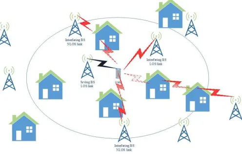
Fig. 1. A schematic of the system model forK= 1. A BS located closer to the origin has a higher chance of LOS propagation. Because of the NLOS path-loss, the signals received from farther BSs are substantially weaker. Nevertheless, the typical UE can still be associated with a BS in NLOS mode due to, for example, fast fading fluctuations.

3

SYSTEM

MODEL

We investigate the downlink communication in a multi-tier cellular network. The network is comprised ofK ≥1tiers of randomly located base stations (BSs), where the BSs of tier i,i∈ K={1, . . . , K}, are spatially distributed according to a homogenous Poisson point process (PPP),Φi, with spatial

density,λi(the number of BSs per unit area),λi ≥0. PPPs,

Φi,Φj,∀i, j∈ K, i6=jare mutually independent. A HetNet

consists ofΦi,i∈ K, i.e.,{Φi}∀i, is referred to asΦ.

UEs are randomly positioned across the network and form a PPP,ΦU, independent ofΦ, with given density,λU.

According to Slivnayak’s Theorem [61], [62] and due to the stationarity of the point processes, the spatial performance of the network can be obtained from the perspective of a typical UE positioned at the origin. We also assume that UEs are equipped withNr_antennas.

Tieriis fully characterized by the corresponding spatial density of BSs, λi, their transmission power, Pi, the

mini-mum required received SIR for the UEs in Tieri, βi ≥ 1,

the number of the transmit antennas at the BSs, Nt i, and

the number of scheduled streams Si ≤ min{Nit, Nr} also

referred to asmultiplexing gain[30], [63], [64]. Fig. 1 shows a schematic model of the network forK= 1.

3.1 Generic LOS/NLOS Path-Loss Model

A block fading wireless channel is considered, where at the beginning of each time slot, an independent realization of the fading is generated and stays fixed throughout that time slot. The typical UE is associated with BSxi, transmittingSi

data streams. The received signal,y_xi ∈CNr_×1

, is

yxi = p

Li(kxik)Hxisxi+ X

j∈K X

xj∈Φj\xi q

Lj(kxjk)Hxjsxj,

(1) where ∀xi, i ∈ K, sxi = [sxi,1. . . sxi,Si]T ∈ CSi×1,

sxi,li ∼ CN(0, Pi/Si)is the transmitted signal

correspond-ing to stream li in Tier i, Hxi ∈ C Nr_×S

i _{is the fading}

channel matrix between BS xi and the typical UE, with

entries independently drawn from CN(0,1). Transmitted

signals across different BSs are also assumed to be mutually independent, and also independent of the channel matrices. In (1), Li(kxik) is a generic distance-dependent path-loss

function, wherekxik is the Euclidean distance between BS

xiand the origin, which is random.

As shown in Fig. 1, a BS experiences LOS or NLOS propagation, depending on its relative distance to the UE, density of buildings, type of the clutter, etc. To model LOS/NLOS pathloss, we adopt the path-loss model recom-mended in the 3rd Generation Partnership Project (3GPP) [16], [17], [18], where the path-loss attenuation in Tieriis

Li(kxik) = (

Li

L(kxik) with probability ofpiL(kxik),

Li

N(kxik) with probability ofpiN(kxik).

(2) For ni ∈ {L,N}, function Lini(kxik) can adopt any

fea-sible path-loss function, e.g., Li

ni(kxik) = φ i nikxik

−αi ni_,

Li

ni(kxik) = φ i

ni(1 + kxik) −αi

ni_{, or L}i_n

i(kxik) =

φi

nimax{1,kxik −αi

ni_{}, where α}i

L (αiN) is the path-loss

ex-ponent associated with the LOS (NLOS) link, φi

L (φiN) is a

constant, characterizing the LOS (NLOS) wireless propaga-tion environment, and is related to various factors, e.g., the height of transceivers, antenna’s beam-width, weather, etc.

In (2), for a BS located at position xi the probability in

LOS mode ispi

ni(kxik), where P

ni∈{L,N}

pi

ni(kxik) = 1. For

instance, ITU-R UMi model is [16], [17]

pi

L(kxik) = min ½

Di

0 kxik,1

¾ ¡

1−e− kxik

Di₁ ¢_+e−

kxik

Di_{1 , (3)}

where, parameters Di

0, andD1i characteriize the near-field

(LOS), and far-field (NLOS) critical distances, respectively. Therefore, if kxik ≤ Di0, BS xi is in LOS mode. For

kxik> Di0, the probability of LOS mode declines

exponen-tially with the distance, and for kxik > Di1, it decreases

quickly to 0.

A similar approach was also adopted in [22], [23], [57] to characterize pi

L(kxik). Note that the model in (3) and

similar approaches in [21], [22], [57] all have a certain level of adjustability to the communication environment (urban, dense urban, or suburban) or the clutter city (flat, scattered, hill-sided, etc.). The critical parameters of these mathemat-ical models, such asDi

0 and D1i in (3), are often obtained

using experimental measurements complemented by data analysis techniques, see, e.g., [57]. Therefore, some of the hidden aspects of channel modeling, such as the correlation in LOS mode—caused by large obstacles/buildings in an area which similarly affect the transmitted signals of adja-cent BSs—are eventually represented in the path-loss model. (It is straightforward to confirm that the SPLM abides by (2).)

For the simulation and numerical studies we consider the path-loss attenuation function, Li

ni(kxik) = φ i ni(1 +

kxik)−α i

ni_{, along with the LOS probability, (3), unless}

3.2 SIR of Data Streams

In the analysis we assume the availability of perfect chan-nel state information at the receiver (CSIR), while CSI at the transmitter (CSIT) is not available. Each BS xi turns

on Si transmit antennas and equally divides its transmit

power,Pi, among them. This transmission scheme is often

referred to as open-loop pre-coding, see, e.g., [63], [64]. At the receiver, the system employs zero-forcing beamforming (ZFBF) [30], [63]. To decode the li-th stream, in ZFBF, a

typical UE uses the available CSIR, Hxi, to mitigate the

inter-stream interference. The typical UE also obtains matrix

(H†xiHxi) −1_H†

xi, where (.)

† _{is the conjugate transpose}

operator, and then multiplies the conjugate of theli-th

col-umn by the received signal in (1). In an interference-limited regime, i.e., ignoring noise, the post-processing SINR asso-ciated with theli-th stream is

SIRxi,li = Pi

SiLi(kxik)H ZF

xi,li

Ili , (4)

where

Ili ∆₌X j∈K

X

xj∈Φj\xi

Pj

SjLj(kxjk)G

ZF

xj,li, (5)

is the inter-cell interference (ICI) streamliexperienced.

As shown in [63], [64], the intended channel power gains associated with the li-th data stream, HxZFi,li, and the ICI

caused byxj 6=xion data streamli,GZFxj,li, are chi-squared

random variables with2(Nr_−S

i+ 1), and2Sj, degrees of

freedom (DoF), respectively. For each li,HxZFi,li and G ZF

xj,li

are independent random variables. For for l 6= li, HxZFi,li

(GZF

xj,li) and H ZF

xi,l (G ZF

xj,l) are independent and identically

distributed (i.i.d.). In (4), for a given communication link,

SIRZF

xi,li, are identical, butnotindependent across streams,

see Section 5.1.

4

COVERAGE

PROBABILITY

MULTI-STREAM

MIMO HETNETS

The coverage probability is defined as the probability that

the SIR stays above a given SIR threshold. The coverage probability in a cellular network is often related to the complementary cumulative distribution function (CCDF) of the received SIR [9], [10], [62]. The same definition is also used in SISO and single-stream MIMO communication systems, e.g., diversity systems and space division multiple access [6], [7]. In multiple stream MIMO, we consider the coverage probability as the probability that all of a typical UE’s streams are successfully decoded at the receiver. Such a notion of coverage probability is also referred to as

all-coverage probabilityin isolated scenarios, e.g., [30], [31], [32],

[33], [65], [66].

4.1 Cell Association

To evaluate the coverage probability, we first need to charac-terize the mechanism used to associate UEs with BSs. This mechanism is often referred to ascell association (CA). De-pending on the communication scenario, application context and signaling structure, two main approaches have been proposed in the literature, including max-SIR [1], [4], [6],

[32], [33], [34], [67], [68], and range expansion (a.k.a. closest-BS) [5], [7], [9].

In the closest-BS (max-CIR) CA, the BS located closest (thus providing the maximum CSI) to the user is considered as the serving BS. Our previous work [14], [34] showed that the coverage performance is substantially improved by adopting max-SIR CA. SIR-based CA is also integrated into various resource-allocation mechanisms by incorporating the physical-layer specifications, transmission policies, and scheduling and coordination across tiers, see, e.g., [36], [69], [70], [71], [72].

4.2 Coverage Probability

In a system with max-SIR, a BS is selected as the serving BS for a typical UE, if all SIRs across the streams are larger than the SIR threshold, βi. Therefore, for a typical UE the

coverage probability of ZFBF is

cZF=P{AZF6=∅}, (6)

where

AZF₌

½

∃i∈ K: max

xi∈Φi min

li=1,...,Si

SIRZF_xi,li ≥βi ¾

. (7)

The NLOS signals are expected to be, on average, weaker than that of LOS. In some cases however, the fading fluctu-ation and the impact of array processing may cause the CA to select a NLOS BSs.

Evaluating cZF_{, for LOS/NLOS, is challenging due to}

the following issues. First, for each data stream, the fading fluctuation in the intended signal is chi-squared, which often results in a less tractable analysis than that of Rayleigh fading. Second, the unconventional LOS/NLOS path-loss model exacerbates the complexity of analysis. Third, the ICI correlation across data streams in a communication link fur-ther interrelates the stream and link coverage probabilities. The cross-stream ICI correlation is created by the existence of the same interferers across data streams, see Section 5.1.

Therefore, conditioned on GZF

xj,li, ∀li, the interference

originated from BS xj, depends on Lj(kxjk), which is a

random variable (r.v.) independent of data stream li. In

[30], [33], we have already developed analytical tools that enable us to deal with the first and the third issues above in cases with SPLM. In what follows, we use this to obtain the coverage probability in cases with the LOS/NLOS path-loss model, addressing the above three issues.

Proposition 1: The coverage probability of a multi-stream MIMO-ZFBF cellular network with LOS/NLOS path-loss, (2), is

cZF=X

i∈K

2πλi N_Xr−Si

m1=0 . . .

N_Xr−Si

m_Si=0

(−1)m1+...+mSi m1!. . . mSi!

∞ Z

0

ridri

∂m1_{. . . ∂}mSi³P

n∈{L,N}p

i n(ri)Ψ

i n(ri)

´

∂tl1m1. . . ∂tl_Si m

lSi

¯ ¯ ¯

t_li=1,∀li ,

where for eachn∈ {L,N},

Ψin(ri) = exp 

_−2πXK j=1

λj ∞ Z

0

yj ¡

1−Ψin(ri, yj) ¢

6

Ψi

n(ri, yj) = X

n0_∈{L,N} pj_n0(yj)

Si Y

li=1

(1 +βiSiPjL

j n0(yj)

SjPiLin(ri) tli) −Si

Proof: See Appendix A. ¥

The coverage probability in Proposition 1 is a function of tiers’ BS densities, their SIR thresholds, transmission powers, and multiplexing gains. The impact of of LOS, and NLOS path-loss for the intended link are captured by functions Ψi_N(ri), and ΨiN(ri), respectively. Furthermore,

ΨiN(ri)andΨ i

N(ri), are functions of the LOS/NLOS modes

of the interfering links, respectively, throughΨi

L(ri, yj), and

Ψi

N(ri, yj).

As a key performance parameter, the coverage probabil-ity is often required to be calculated many times in various resource-allocation schemes to find the best combination of the network operational parameters. Calculating the cov-erage probability in Proposition 1 is, however, challenging due to the requirement of extensive numerical calculations. Thus, we propose several approximations of the coverage probability with acceptable accuracy and reasonable com-putational complexity.

5

COVERAGE

PROBABILITY

APPROXIMATION

The link-level coverage probability, as defined in Section 3, is directly related to the SIR of every single stream in that link. The SIR values for streams are, however, strongly correlated due to cross-stream ICI correlation. Therefore, to evaluate the coverage probability, we first need to quantify the cross-stream ICI correlation.

5.1 Cross-Stream ICI Correlation

We use Pearson correlation coefficients to characterize the ICI correlation between streamsli6=li0:

ρli,l0i=

E[IliIl0i]−E[Ili]E[Il0i] p

Var(Ili)Var(Il0i)

, (8)

where Var(x) is the variance of random variable x. We further note that the ICI is an identical shot-noise process across streams, soρli,l0i is

1

ρli,l0i =

E[Ili_Il0i]−(E[Ili_])2

Var(Ili) . (9)

Proposition 2: For a MIMO-ZFBF multiplexing system with the generic LOS/NLOS pathloss,

ρli,l0i=

P

j∈K

P2

jλj P

nj∈{L,N} ∞ R

0

rjpjnj(rj)(L j nj(rj))

2_dr

j P

j∈K

P2

j

Sj(Sj+1)−1 S2

j λj P

nj∈{L,N} ∞ R

0

rjpjnj(rj)(L j

nj(rj))2drj

.

(10)

Proof: See Appendix B. ¥

1. Interference correlation is studied in [50], [62], [73], focusing on quantifying the impact of interference correlation on the time and receive-array diversities. Here we are interested in quantifying the impact of multiplexing gains and NLOS/NLOS path-loss model on the interference correlation. We also use this analysis to corroborate the validity of the full-correlation (FC) assumption for approximating the coverage probability.

For a single tier network,K= 1, Proposition 2 results in the following corollary.

Corollary 1: For a single tier MIMO-ZFBF,

ρl1,l01 =

S2 1

S1(S1+ 1)−1, (11)

which only depends on the multiplexing gain.

Proposition 3: In a MIMO-ZFBF multiplexing system,

0.5≤ 1 1 + maxiSi_S−21

i

≤ρli,l0i ≤

1 1 + miniS_Si−21

i

≤1. (12)

Proof: See Appendix C. ¥

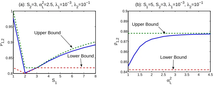
Proposition 3 shows that in the MIMO multiplexing system,ρli,l0i is larger than 0.5, so ICI is highly correlated

across data streams. In Fig. (2-a), we illustrateρl1,l01vs.S1for

a simulated system. ICIs across data streams are shown to be significantly correlated. Fig. (2-a) also confirms the validity of the bound in Proposition 3.

Also, Fig. (2-a) shows that forS1 >2(S1 <2),ρl1,l01 is

an increasing (decreasing) function ofS1, and its maximum

(minimum) occurs atS1 = 2. Setting the derivative of (??)

to zero, one can analytically obtainS1= 2:

∂ρl1,l01

∂S1 =

P

j∈K

λjAj Ã

P

j∈K

λjAjSj(Sj_S+1)2 −1 j

!2

S1(S1−2)

S4 1

= 0. (13)

In Fig. (2-b), we present ρl1,l01 vs. α 2

L. ρl1,l01 in (2-b) is

shown to vary within the bounds given in Proposition 3. Fig. (2-b) shows ρl1,l01 to be also highly correlated across

streams, and an increasing function ofα2

L. This is also stated

in the following corollary. Corollary 2: Increasing α2

L results in a higherρl1,l01 for

any combination of multiplexing gains for which

X

j∈K

λjAjSj(Sj+ 1)−1

S2

j

>S2(S2+ 1)−1 S2

2

X

j∈K

λjAj. (14)

Proof:See Appendix D. ¥

The system considered for the simulation in Fig. (2-b) is a two-tier system,K= 2. For this system (14) is reduced to:

S1(S1+ 1)−1

S2 1

> S2(S2+ 1)−1 S2

2

,

which holds ifS1 > S2 >2.2That is, for anyS1 > S2 >2,

∂ρl₁,l0

1 ∂α2

L >0.

5.2 Full Correlation Assumption

Our analysis in Section 5.1 indicates that the ICI is highly correlated across the streams, justifying the construction of ’full-correlation‘ (FC) approximation, where the ICI across all streams in a given communication link is considered fully correlated, i.e.,ρli,l0i = 1. Such an assumption has also been

used for analyzing other aspects of MIMO systems in [32], [33], [43].

1 2 3 4 5 6 7 8 0.8

0.85 0.9 0.95 1

(a): S 2=3, αL

2 =2.5, λ

1=10 −3

, λ 2=10

−1

S 1

ρ 1,2

Upper Bound

Lower Bound

1 1.5 2 2.5 3 3.5 4 4.5 0.84

0.85 0.86 0.87 0.88 0.89 0.9

α_L2

ρ1,2

(b): S

1=5, S2=3, λ1=10 −3

, λ 2=10

−1

Upper Bound

Lower Bound

Fig. 2. Cross-stream ICI correlation coefficient vs.S1,α2

L, the simulation results and bounds, in a system withK= 2,α1N = 3.75,α2N = 4.75,

P1= 25W,P2= 1W,N1t= 16,N2t= 8,Nr= 8,D01= 36,D20= 9,D11= 48,D21= 18meter, andφiL=φiN= 1.

Assuming FC, ICI for the typical UE associated with BS xiis

IFC₌X

j∈K X

xj∈Φj\xi

Pj

Sj

Lj(kxjk)GZFxj, (15)

where forli= 1,2, . . . , Siwe simply replace the interfering

channel power gain,GZF

xj,li, withG ZF

xj (both chi-squared r.v.s

with2Sj DoFs). For data streamli, the post-processing SIR

is then approximated as

SIRZFxi,l−iFC= Pi

SiLi(kxik)H

ZF

xi,li

IFC . (16)

Therefore, for the max-SIR CA under the FC assumption, the max-SIR CA rule 7 is rewritten as

AZF−FC=

(

∃i∈ K: max

xi∈Φi P_i

SiLi(kxik)H

ZF

xi,min IFC ≥βi

)

, (17)

HZF

xi,min ∆

= min

li=1,...,Si

HZF

xi,li. This implies that the

prob-ability of coverage for the typical UE is cZF−FC ₌

Pr©AZF−FC_6=∅ª_{. Similarly to Appendix A, we then use}

Lemma 1 in [4] to derive the coverage probability as

cZF−FC_=P  

Smax

i∈K

xi∈Φi Pi

SiLi(kxik)H

ZF

xi,min IFC ≥βi

 



=X

i∈K

E X

xi∈Φi

1

Ã_P

i

SiLi(kxik)H

ZF

xi,min IFC ≥βi

!

=X

i∈K

2πλi

∞ Z

0

riP

(_P

i SiLi(ri)H

ZF

xi,min IFC ≥βi

)

dri

=X

i∈K

2πλi

∞ Z

0

riELi(ri),Φ,{Lj(kxjk)}∀xj ,jP

n

HxZFi,min≥

βiIFC Pi SiLi(ri)

¯

¯_{Φ, Li(ri),{Lj(kxjk)}∀x}

j,j

o

dri. (18)

Evaluating the coverage probability based on (18) is shown to be a complicated task. To address this difficulty, we propose two approximations for (18) which enable the nu-merical evaluation of the coverage probability as a function of the main system parameters.

5.2.1 Alzer Approximation

Alzer’s inequality [56], [57] (see Appendix-C Lemma 1) has been used to evaluate the coverage probability under Nakagami-type fading and multi-user MIMO systems using stochastic geometry. Here, for the first time we extend Alzer’s inequality to approximate the coverage probability of a multi-stream multi-tier MIMO-ZFBF system. We refer to this method as A-A, where Alzer’s lemma is utilized to approximate the effective power gain of the attending channel for each data stream as an exponential random variable. This is presented in the following Proposition.

Proposition 4: In a multi-stream MIMO-ZFBF

cellu-lar system with LOS/NLOS pathloss model, and S0

i =

((Nr_−S

i+ 1)!)− 1

(N r−Si+1)_{, the coverage probability is}

ap-proximated as

cA−A₌X

i∈K

2πλi

Ã

1 +

Si

X

l0

i=1

(Nr−_XSi+1)l0i

l00

i=0

(−1)l0_i+l00_i×

Ã

(Nr_−S i+ 1)li0 l00

i

!Ã

Si l0

i

! X

ni∈L,N

∞ Z

0

ripin_i(ri)Ψbin_i(ri)dri

!

, (19)

where Ψbi

n_i(ri) = exp

Ã

−2πP

j λj

∞ R

0

yj(1−Ψbin_i(ri, yj))dyj

! ,

b

Ψini(ri, yj) = X

nj∈{L,N}

pj nj(yj) ¡

1 +S0 il00i

βiSiPjLjnj(yj) SjPiLi_ni(ri)

¢Sj

.

Proof:See Appendix E. ¥

The numerical complexity of obtainingcA−A_in

Propo-sition 4 is significantly lower than that of PropoPropo-sition 1 as there are no concatenated higher-order differentiations. The impact of LOS/NLOS model parameters on the intended and interfering links can be seen in Ψbi

L(ri)/ ΨbiN(ri), and b

Ψi

L(ri, yj)/ΨbiN(ri, yj).

5.2.2 Gamma Approximation The coverage probability,cZF−FC_{, is}

cZF−FC=X

i∈K

2πλi X

ni∈L,N ∞ Z

0

8

0 50 100 150

0 0.2 0.4 0.6 0.8 1 x CDF

sim. αL 2

=1.5

Gamma fit αL 2

=1.5

sim. αL 2

=2.09

Gamma fit αL 2

=2.09

sim. αL 2

=4

Gamma fit αL 2

=4

0 5000 10000 15000

0 0.2 0.4 0.6 0.8 1 x CDF

sim. S1=4

Gamma fit S1=4

sim. S1=1

Gamma fit S

1=1

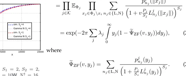
Fig. 3. CDF of _IFC1 , (a):λ1 = 10−4,λ2 = 10−3,S1 = 2,S2 = 2,

α1

L= 2.09,α1N = 3.75,α2N= 4.75,P1 = 50W,P2 = 10W,N1t = 16,

Nt

2 = 8,Nr = 8, andφiL = φiN = 1; (b)λ1 = 10−4, λ2 = 10−3,

S2 = 2,α1L = 2.09,α1N = 3.75,α2L = 1.5,αN2 = 4.75,P1 = 50W,

P2= 10W,N1t= 16,N2t= 8,Nr= 8, andφiL=φiN= 1.

EIFCP (

HZF

xi,min

IFC ≥

βi Pi SiL

i ni(ri)

¯ ¯_{Φ, I}FC

)

dri. (20)

Instead of the intended fading gain, one may approximate the statistical characteristics ofIFC_{. Note, however, that in}

the max-SIR CA, in some cases the interferers are even closer to the typical UE than the serving BS. This can happen, for instance, in LOS mode with a very small LOS path-loss ex-ponent. For LOS path-loss functions, whereLi

L(x)∝x−α i L,

the mean and variance ofIFC _{could be very high. Instead,}

we model _IFC1 .

The CDF of _IFC1 is plotted in Fig. (3) for the simulated

system with the parameters given in the caption. Fig. (3-a) shows that for different values of the LOS path-loss exponent, the CDF closely follows the Gamma distribution. Fig. (3-b) further shows that the approximation based on Gamma distribution remains valid for various multiplexing gains. This has also been confirmed for a variety of other system parameters which are not reported here due to space limitation.

Based on the above, we approximate the CDF of 1

IFC

by a Gamma distribution, 1

IFC ∝ Gamma(a, b), where,

adopting a moment-matching technique, parametersaand

bare obtained as

a= (E

1

IFC)2 (E 1

(IFC₎2−(E_IFC1 )2)

, (21)

b= E

1

IFC (E 1

(IFC₎2 −(E_IFC1 )2)

. (22)

For aGamma(a, b)random variable with pdf fX(x) = ba

Γ(a)xa−1e−bx,X = ab andVar(X) = ba2. To obtainaandb,

we need to calculateE 1

IFC andE_(IFC1₎2. The former is given

by

E 1

IFC =E

∞ Z

0

e−vIFCdv=

∞ Z

0

e

Ψ(v)dv, (23)

whereΨ(e v)is the Laplace transform ofIFC_:

e

Ψ(v) =Ee

−v P j∈K

P

xj∈Φ_j\xi Pj

SjLj(kxjk)GZF_xj

= Y

j∈K EΦj

Y

xj∈Φj\xi EGZF

xj,Lj(kxjk)e

−vPj_SjLj(kxjk)GZF_xj

= Y

j∈K EΦj

Y

xj∈Φj\xi X

nj∈{L,N}

pj

nj(kxjk) ³

1 +vPj SjL

j nj(kxjk)

´Sj

= exp(−2πX

j

λj ∞ Z

0

yj(1−ΨZF(e v, yj))dyj), (24)

where

e

ΨZF(v, yj) = X

nj∈L,N

pj nj(yj) ³

1 + Pj SjL

j nj(yj)

´Sj. (25)

Note that inΨZF(e v, yj, Sj) the first (second) term is

asso-ciated with the LOS (NLOS) mode of the BS located atyj.

Similarly, the second moment of _IFC1 is:

E 1

(IFC₎2 =E

∞ Z 0 ∞ Z 0

e−(v1+v2)IFC_dv 1dv2=

∞ Z 0 ∞ Z 0 e

Ψ(v1+v2)dv1dv2=

∞ Z

0

vΨ(e v)dv. (26)

Using the above, in the following we approximate the coverage probability using Gamma distribution, which will henceforth be called G-A.

Proposition 5:We define

X

i,k ∆

= X

k0+k2+...+kN r−Si=Si−1 µ

Si−1

k0, k2, . . . , kNr_−S i

¶

,

andS˜i(k) =∆ Nr−Si+ 1 + Nr_−S

i P

l=0

lkl. An approximation,

namely G-A, of the coverage probability in a multi-stream MIMO-ZFBF cellular network with an LOS/NLOS attenua-tion, (2), is

cG−A₌X

i∈K

2πλiSi

(Nr_−Si)!Γ(a) X

ni∈{L,N} X i,k × ∞ Z 0 ∞ Z 0

ripini(ri)

hS˜i(k)−1_e−Sih Nr_−S

i Q

l=0 (l!)kl

γ

Ã

a, b_P βi

i SiL

i ni(ri)h

!

dridh

(27) whereγ(a, bx)is the CDF of random variableGamma(a, b).

Proof: See Appendix F. ¥

Compared to Proposition 1, in Proposition 4 the numer-ical complexity of obtaining an approximation of the cov-erage probability is substantially reduced. Nevertheless, the numerical complexity of obtainingcG−A_{is higher than that}

ofcA−A_{, because in G-A,aand bshould also be obtained}

as in (21) and (22), respectively. G-A further requires the calculation of double integration which is not required in A-A, see (46).

In G-A, a and b are tier-independent—once they are

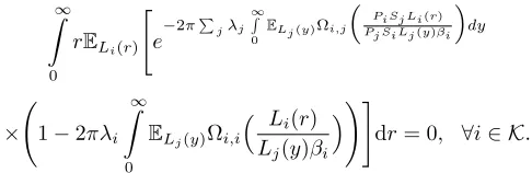
The simulation results in Section 7 reveal that the extra complexity of G-A brings a higher accuracy and robustness over a wide range of system parameters. Compared to A-A, G-A also captures the actual behavior of the coverage probability against densification more precisely. Further, as shown in Section 7, G-A enables accurate evaluation of BSs’ density for which the maximum coverage performance is achieved.

6

SPECIAL

CASES

We use the results derived for open-loop ZFBF MIMO multiplexing system to evaluate the coverage performance in MIMO diversity only, ZFBF with nonhomogeneous and homogenous SPLM, and systems with available CSIT (full CSIT and quantized CSIT). The main objective is to demon-strate how one can derive the coverage probability of vari-ous MIMO system settings using the analytical framework developed in this paper. The analytical results here are supported further by the simulations and numerical results in Section 7.

6.1 Diversity Only Systems

In this type of systems,Si= 1,∀i, i.e., single-stream MIMO

or single-input multiple-output (SIMO) systems.

A-A Method:Proposition 4 is reduced to

cSIMO−A−A=X

i∈K

2πλi Ã

1 +Si Nr X l00 i=0 µ Nr l00 i ¶

(−1)l00i+1

X

ni∈{L,N} ∞ Z

0

ripini(ri)Ψb i

ni(ri)dri !

, (28)

whereΨbi

ni(ri)is defined as

b

Ψi

ni(ri, yj) = X

nj∈{L,N}

pj nj(yj) µ

1 + (Nr_!)− 1

N rl00_i βiPjL j nj(yj) PiLi_ni(ri)

¶Sj.

G-A Method: Using Proposition 5, G-A approximation

implies that

cSIMO−G−A₌X

i∈K

2πλi

(Nr_−1)!Γ(a) X

ni∈{L,N}

× ∞ Z 0 ∞ Z 0

ripini(ri)h Nr₋₁

e−h_γ µ

a, b βi

PiLini(ri)h ¶

dridh,

(29) where

a= (E

1

IFC)2 (E 1

(IFC₎2−(E_IFC1 )2)

, (30)

b= E

1

IFC (E 1

(IFC₎2 −(E_IFC1 )2)

, (31)

and

E 1

IFC =

∞ Z

0

exp(−2πX

j

λj ∞ Z

0

yj(1−ΨD(e v, yj))dyj)dv,

(32)

E 1

(IFC₎2 =

∞ Z

0

vexp(−2πX

j

λj ∞ Z

0

yj(1−ΨD(e v, yj))dyj)dv,

(33) whereΨD(e v, yj)is defined similarly to (25), whereSj = 1.

6.2 ZFBF Multiplexing with Non-homogeneous SPLM

In non-homogeneous SPLM,αi

L=αiN =αi andφiL =φiN,

∀i.

A-A Method: It is straightforward to show that the

ap-proximation of the coverage probability based on A-A is

cA−A=X

i∈K

2πλi

à 1 + Si X l0 i=1

(Nr−_XSi+1)l0i

l00

i=0

Ã

(Nr_−S i+ 1)l0i l00

i

!

(−1)l0i+l00i

Ã

Si l0

i

!_Z∞

0

rie

−2πP j

λj W(αj)r 2αi

αj i

αj(S_il000_i βiSiPj Pi )

2+ 2 αj

dri, (34)

whereW(αj) = ∞ R

0

w−1−αj2 _(1−e−w_)dw.

G-A Method:Using Proposition 5,

cG−A=X

i∈K

2πλiSi

(Nr_−S i)!Γ(a)

X i,k × ∞ Z 0 ∞ Z 0

rih

˜

Si(k)−1_e−Sih Nr_−S

i Q

l=0 (l!)kl

γ

Ã

a, bβir

αi i Pi Sih

!

dridh, (35)

where parameters a and b are defined, respectively, in

(30) and (31). To derive these parameters, we should re-place ΨZF(e v, yj)in (25) with ΨZFe −Nonhomogeneous(v, yj) =

1

µ

1+Pj_Sjy_j−αj

¶

Sj, along with (32) and (33).

6.3 ZFBF Multiplexing with Homogeneous Standard

Path-Loss Model

In Homogeneous SPLM,αi=α∀i.

A-A Method: One may start with (34) and apply a

straightforward integration, to show that the coverage prob-ability is approximated as

cA−A= α

W(α)P

j

λjPjαˇ X

i∈K

λi(_βP_iSi_i)2+ ˇα

(S0 i)2+ ˇα

à 1+ Si X l0 i=1 (Nr_−S

i+1)l0i X

l00

i=0

(−1)l0

i+l00i µ

Si

l0 i

¶µ

(Nr_−S i+ 1)l0i

l00 i

¶

l002+ ˇα i

!

.

This expression is similar to the upper-bound provided in Proposition 1 in [30]:

cZF_≤ π

˜

C(α)

X i∈K λi ³ Pi S2

iβi

´αˇµNr_−S i P

ri=0 Γ(αˇ

Si+ri) Γ(αˇ

Si)Γ(1+ri) ¶Si

P j∈Kλj

³ Pj Sj

´αˇµ_Γ(αˇ Si+Sj) Γ(Sj)

¶Si ,

10

G-A Method:Proposition 5 yields:

cG−A₌X

i∈K

2πλiSi

(Nr_−Si)!Γ(a) X

i,k

×

∞ Z

0

∞ Z

0

rih

˜

Si(k)−1e−Sih Nr_Q−Si

l=0 (l!)kl

γ

Ã

a, bβirαi Pi Sih

!

dridh, (37)

where parameters a and b are defined in (30) and (31),

respectively. To derive these parameters, we setΨZF(e v, yj)

in (25) withΨZFe −Homogeneous(v, yj) = µ 1

1+Pj_Sjy−α j

¶

Sj, along

with (32) and (33).

6.4 Known CSIT

In the above derivations, we simply assume that the CSIT is not known to the BSs. However, there are practical scenarios that CSIT is available to BSs. So, our analysis is shown to cover such cases as well.

6.4.1 Single-Input Single-Output (SISO) Systems

For a SISO system,Si = Nit =Nr = 1and Proposition 1

yields:

cSISO=X

i∈K

2πλi X

n∈{L,N} ∞ Z

0

ripin(ri) exp(−2π K X

j=1

λj

∞ Z

0

yj ¡

1−Ψn(ri, yj) ¢

dyj)dri,

where

Ψn(ri, yj) =

X

n0∈{L,N}

pj_n0(yj)(1 +

βiPjLjn0(yj) PiLin(ri) )

−1

.

Note that for this scenario, both A-A and Proposition 1 yield the same coverage performance.

G-A Method:Using Proposition 5,

cSISO−G−A₌X

i∈K

2πλi

Γ(a)

X

ni∈{L,N}

×

∞ Z

0

∞ Z

0

ripini(ri)e −h_γ

µ

a, b βi

PiLini(ri)h ¶

dridh, (38)

wherea, andbare defined in (30), and (31), respectively. To derive these parameters, one should replace ΨZF(e v, yj) in

(25) with ΨSISO(e v, yj) = P

nj∈L,N pj

nj(yj)

(1+PjLj_nj(yj)), along with

(32) and (33).

6.4.2 Multiple-Input Single-Output (MISO) Systems In a MISO system,Nr _{= 1, andS}

i= 1,∀i. We assume that

available CSIT at the BSs is utilized for eigen-beamforming, i.e., maximum ratio transmission (MRT) [74]. In this system, the SIR at the typical UE served by BSxiis

SIRMRTxi =

PiLi(kxik)HxMRTi

P

j∈K P

xj∈Φj/xi

PjLj(kxjk)GMRTxj

, (39)

where HMRT

xi andG MRT

xj are chi-squared with 2N t

i DoFs,

and exponential random variables, respectively.

A-A Method:Using Proposition 4,

cMRT−A−A₌X

i∈K

2πλi Ã

1 +

Nr X

l00

i=0 (−1)l00

i+1

µ

Nr

l00 i

¶ X

ni∈L,N ∞ Z

0

ripini(ri)Ψb i

ni(ri)dri !

, (40)

where Ψbi

ni(ri) = exp(−2π P

j

λj ∞ R

0

yj(1−Ψbini(ri, yj))dyj),

and,

b

Ψi

L(ri, yj) = X

nj∈{L,N}

pj nj(yj) µ

1 + (Nr_!)− 1

N rl00_iβiPjL j nj(yj) PiLi_ni(ri)

¶Sj.

G-A Method:Using Proposition 5,

cSIMO−G−A₌X

i∈K

2πλi

(Nr_−1)!Γ(a) X

ni∈{L,N}

×

∞ Z

0

∞ Z

0

ripini(ri)h Nr₋₁

e−h_γ µ

a, b βi

PiLini(ri)h ¶

dridh,

(41) whereaandbare obtained by replacingΨZF(e v, yj)in (25)

withΨSIMO(e v, yj) = P

nj∈L,N pj

nj(yj)

(1+PjLjnj(yj)), along with (32)

and (33).

6.4.3 MISO-SDMA Systems

Another instance is when the BSs have access to CSIT in

an MISO-SDMA system. Here Nr _{= 1, and S}

i = 1, ∀i.

We further assume that each cell of tier iserves Ui ≤ Nit

UEs using ZFBF at the transmitter, see, e.g., [6], [7] for more details. Assuming a fixed transmit power, the SIR of the typical UE associated with BSxiis

SIRSDMAxi =

Pi

UiLi(kxik)H SDMA

xi P

j∈K P

xj∈Φj/xi Pj

UjLj(kxjk)G SDMA

xj

, (42)

where HSDMA

xi and G SDMA

xj are both chi-squared random

variables with2(Nt

i −Ui+ 1)and2Uj DoFs, respectively

[6], [14].

A-A Method:Using Proposition 4,

cSDMA−A−A₌X

i∈K

2πλi Ã

1 +

Nr_l0

i X

l00

i=0 (−1)l00

µ

Nr_l0 i

l00 i

¶ X

ni∈L,N ∞ Z

0

ripini(ri)Ψb i

ni(ri)dri !

, (43)

where Ψbi

ni(ri) = exp(−2π

P

j λj

∞ R

0

yj(1−Ψbini(ri, yj))dyj), in

which,

b

Ψi

ni(ri, yj) = X

nj∈{L,N}

pj nj(yj) ¡

1 +U0 il00i

βiUiPjLjnj(yj) UjPiLi_ni(ri)

¢Uj

.

G-A Method:Using Proposition 5, the G-A approximation

is

cSIMO−G−A₌X

i∈K

2πλi

(Nr_−Ui)!Γ(a) X

ni∈{L,N}

×

∞ Z

0

∞ Z

0

ripini(ri)h Nr_−U

i_e−h_γ Ã

a, b_P βi

i UiL

i ni(ri)h

!

dridh,

(44)

where parameters a and b are obtained by

re-placing ΨZF(e v, yj) in (25) with ΨSDMA(e v, yj) = P

nj∈L,N pj

nj(yj)

µ

1+_UjPjLj nj(yj)

¶_Uj along with (32) and (33).

6.5 Imperfect CSIT

In practice, instead of a perfect CIST, often a delayed and/or quantized version of channel directional information (CDI) is available at the BSs. Consider the MISO-SDMA system

discussed above, and assume UEs report CDI using Bi

feedback bits associated with tier i. Following the same line of argument as in [75], [76], [77], we can obtain the received channel power and interference statistics. Never-theless, based on imperfect CDI, zero-forcing beamforming is unable to completely eliminate the inter-user interference. Therefore, assuming quantization cell approximation (QCA) [75], [77], [78], the SIR of the typical UE associated with BS xiis :

SIRQSDMAxi ≈ (45)

Pi

UiLi(kxik)H SDMA

xi (1−φi) Pi

UiLi(kxik)G QSDMA

xi φi+ P

j∈K P

xj∈Φj/xi Pj

UjLj(kxjk)G SDMA

xj

,

where φi = 2

− Bi

N t_i−1 _{and G}QSDMA

xi is an exponentially

distributed random variable with unit mean and

indepen-dent of HSDMA

xi and G SDMA

xi [77], [78]. Note that the SIR

expression in (45) is in fact an approximation derived based on QCA. Therefore, assuming exponential distribution for

random variable,GQSDMA

xi , highly relies on QCA and may

become inaccurate if this assumption does not hold. Never-theless, as our simulations also suggest, the QCA assump-tion provides a high level of accuracy, and therefore (45) is rather a close approximation.

For a system with imperfect CDIR, we obtain the outage probability using A-A and G-A methods.

A-A Method:

Using Proposition 4,

cQSDMA−A−A₌X

i∈K

2πλi Ã

1 +

Nr_l0

i X

l00

i=0 (−1)l00

i+1

µ

Nr_l0 i

l00 i

¶ X

ni∈L,N ∞ Z

0

ripini(ri)Ψb i ni(ri) 1 +U0

il00i PUiiL i ni(ri)φi

dri !

, (46)

where Ψbi

ni(ri) = exp(−2π

P

j λj

∞ R

0

yj(1−Ψbini(ri, yj))dyj), in

which,

b

Ψi

ni(ri, yj) = X

nj∈{L,N}

pj nj(yj) ¡

1 +U0 ili001−φβii

UiPjLjnj(yj) UjPiLi_ni(ri)

¢Uj

.

G-A Method:

Using Proposition 5, the G-A approximation is

cQSDMA−G−A=X

i∈K

2πλi

(Nr_−U i)!Γ(a)

X

ni∈{L,N}

×

∞ Z

0

∞ Z

0

ripini(ri)h Nr_−U

i_e−h

1 + Pi UiL

i ni(ri)φi

γ

Ã

a, b

βi (1−φi) Pi UiL

i ni(ri)h

!

dridh,

(47) whereaandbare obtained by replacingΨZF(e v, yj)in (25)

with ΨSDMA(e v, yj) = P

nj∈L,N pj

nj(yj)

µ

1+Pj UjL

j nj(yj)

¶_Uj along with

(32) and (33).

From the above analysis, one can see that an imper-fect CSIT increases the SIR threshold from βi to _1−φβi_i.

Imperfect CSIT also creates extra interference—inter-user interference— but the level of this extra interference is reduced by increasingBi.

7

SIMULATIONS AND

NUMERICAL

ANALYSIS

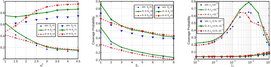
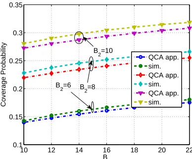
We first evaluate the accuracy of the proposed approxima-tions of the coverage probability. We then study the effects of various system parameters on the coverage probability as well as area spectral efficiency (ASE) to gain insight on the effects of densification, multiplexing gains, and propagation environment.

The simulation results are based on the Monte Carlo simulation, where 40,000 snap-shots are independently sim-ulated and averaged. In each snap-shot, we randomly create BSs based on the given densities in a disk with radius of 10,000 units. The fading matrices are then randomly generated for each snap-shot based on a Rayleigh fading distribution. The LOS/NLOS path-loss for each BS is also specified based on the probabilistic model in (3). System parameters are set as: P1 = 25 W,P2 = 1 W,N1t = 16,

Nt

2 = 8, Nr = 8, β1 = 5,β2 = 2.5,D01 = 36, D20 = 9,

D1