Pau Vilimelis Aceituno∗
Max Planck Institute for Mathematics in the Sciences, 04103 Leipzig, Germany
Tim Rogers†
Centre for Networks and Collective Behaviour, Department of Mathematical Sciences, University of Bath, Bath, BA27AY, UK
Henning Schomerus‡
Department of Physics, Lancaster University, Lancaster, LA1 4YB, UK
The celebrated elliptic law describes the distribution of eigenvalues of random matrices with correlations between off-diagonal pairs of elements, having applications to a wide range of physical and biological systems. Here, we investigate the generalization of this law to random matrices exhibiting higher-order cyclic correlations between k-tuples of matrix entries. We show that the eigenvalue spectrum in this ensemble is bounded by a hypotrochoid curve with k-fold rotational symmetry. This hypotrochoid law applies to full matrices as well as sparse ones, and thereby holds with remarkable universality. We further extend our analysis to matrices and graphs with competing cycle motifs, which are described more generally by polytrochoid spectral boundaries.
Determining the eigenvalue spectra of large random matrices is a rich theoretical problem [1] with many ap-plications in fields as diverse as telecommunications [2], quantum physics [3], ecology [4, 5] and economics [6]. A key result in this field is the elliptic law [7], which states that in the limit of large matrix size the eigenvalues for random matrices with correlations between symmetric pairs of entries are confined within an ellipse in the com-plex plane. This result originating from over 30 years ago still drives scientific developments today, in both mathe-matical theory [8–12] as well as applications [5, 13].
As the applications of random matrix theory have di-versified, so too have the ensembles under study. Existing generalizations of the elliptic law fall broadly into three categories. There is a large body of theoretical work con-cerning random matrix ensembles defined by potential functions, where the quadratic case recovers the elliptic law, but more complicated potentials produce interesting spectral distributions (see e.g. [14, 15]). Alternatively, for some applications it is necessary to impose a system-level structure such as modularity (see e.g. [16]), often by addition or multiplication with another matrix; see [17, 18] for methods and rigorous mathematical results. Lastly, growing interest in the study of complex networks has led many authors to consider sparse ensembles con-taining many zero matrix elements, where the location of the non-zero elements encodes the adjacency matrix of some directed graph (ordigraph), and can have strik-ing eigenvalue distributions [19, 20] (see [21] for a recent topical review). In none of these directions of work has the problem of high-order correlations been fully and di-rectly addressed. This is not for lack of interest. Multi-party interactions in dense systems are important in bi-ological applications such as ecology [22], stabilization of microbial communities [23] or gene–gene interactions [24] and can provide valuable engineering insights into machine learning [25, 26] and control theory [27].
More--1 0 1
-1 0 1
-2 0 2
[image:1.612.320.557.285.395.2]-2 -1 0 1 2
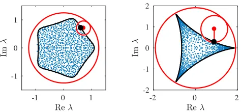
FIG. 1. Hypotrochoid curves (black lines) bounding the eigen-value spectra (blue dots) of random matrices with higher-order correlations. Left: a dense N ×N random matrix M with TrM5/N = 0.075 and other correlations negligible. Right: a random digraph in which each node appears in ex-actly two directed cycles of length three, with no other edges. In both casesN = 1000. The large and small red circles re-spectively show the fixed and rotating wheels describing the hypotrochoid curve.
over, most of the sparse random matrix literature hinges on the assumption of atree-like interaction structure; it remains a long-standing and important problem to allow the relaxation of this assumption, inducing higher-order correlations.
case where more than one correlation order is present, we find a more general family of polytrochoid boundary curves described by multiple linked gears [28].
Dense matrices.—We studyN ×N-dimensional non-hermitian matrices with real or complex entries indepen-dently drawn from a distribution with zero mean and bounded variance. For any of such matrix M, the den-sityµ(z) of complex eigenvaluesz can be obtained from a Green’s function of the form [17, 29, 30]
G(z, z∗) =
z11−M iλ11 iλ11 z∗11−M†
−1 ≡
G11 G12
G21 G22
, (1)
where z∗ denotes complex conjugation and M† the ad-joint; for a real matrix this is just the transpose. Thereby
µ(z) = 1 π
∂g11
∂z∗, (2)
g(z, z∗) = lim
λ→0+
TrG11 TrG12 TrG21 TrG22
≡
g11 g12
g21 g22
.
For a random matrixM, the ensemble-averaged density µ(z) therefore follows fromg(z, z∗).
This can be used to derive the elliptic law of random matrices in the large N limit, which serves as useful preparation. Let us expand
G=Z−1 ∞ X
`=0
(MZ−1)` (3)
into a geometric series, where
Z=Z⊗11, Z =
z iλ iλ z∗
, M=
M 0 0 M†
. (4)
When we perform the averaging, only certain products of matrix elements Mnm survive. These can be
organ-ised into groups of terms whose number scales differently in the matrix dimension N. In particular, there will be many terms where we can pair Mnm with (M†)mn
to yield a finite average. If no further correlations are present the leading order is
G=Z−1+Z−1MGMG, (5)
where the lines denote a pair of matrices that are av-eraged. This factorization of the average is called the non-crossing or planar approximation. It enjoys a large degree of universality based on combinatorial arguments, going much beyond the case of Gaussian statistics where the indicated pairings represent Wick contractions, which are embodied in the framework of free probability [30].
The elliptic law is derived straightforwardly from the expression above. Carrying out the average of the M matrices, taking the partial trace on both sides, and re-arranging forZ, one obtains
Z=N/g+
τ22g11 σ2g12
σ2g21 τ22g22
. (6)
Comparing terms in the off-diagonal in this equation (and noting the constraints ¯g11 = ¯g22∗ and g12 =g21 >0), we find two possible solutions: (i) either g12 = 0, or (ii) |¯g11|2−g¯2
12=N/σ2. The first of these yields ¯g11 propor-tional tozand therefore holds only outside of the support of the spectrum. Examining the diagonal elements of (6) in the case (ii) we obtain
z=σ2g∗11+τ22g11. (7)
which must be solved together with the constraint that |¯g11|2−N/σ2 > 0. The boundary of the spectrum is therefore found by determining the values ofz for which |¯g11|2 = N/σ2; in the present case one finds an ellipse with foci±2τ2
√
N. Inside the support, one can solve (7) to determineg11 and apply (2) to find that the spectral densityµ(z) is uniform.
To generalize these results to ensembles with high-order correlations where TrMk/N is a fixed parameter,
we reinterpret the Hermitian contributions of weightτ2in the elliptic law as correlations of orderk= 2. Introduc-ing correlations of general orderk, we pick up additional contributions corresponding to contractions
G=Z−1+X
k
Z−1(MG)k−1MG, (8)
where k matrices are combined by the indicated lines. Our results will show that these contributions rise to a notable departure from the universal elliptic law, there-fore, constitute the relevant perturbations beyond estab-lished theory. We assume for now that there is just a single extra term of these, of fixedkand with weightτk.
This gives
Z=N/g+
τkkgk11−1 σ2g12
σ2g21 τkkg k−1 22
(9)
and results, inside the spectrum, in the equations
z=σ2g∗11+τkkgk11−1,
g212=|g11|2−N/σ2. (10)
The boundary of the support is therefore determined by the condition |g11|2 = N/σ2. In the large N limit we choose the scalingsσ2 =N−1, τk
k =ρkN1−k to balance
the contribution of terms in (10). With the parameter-ization g11 = N eiϕ, which we insert into Eq. (10), the
boundary curve then becomes
zb(ϕ) =e−iϕ+ρkei(k−1)ϕ. (11)
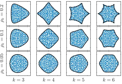
FIG. 2. Hypotrochoid curves (black lines) bounding the eigen-value spectra (blue dots) of random matrices with correlations TrMk=N ρ
k.
Note that (although hard to determine from Fig. 2), for k >2 the density of eigenvalues inside the hypotrochoid support is in fact not uniform; in general solutions to (10) do not have the property that∂g¯11/∂z∗is constant. This distribution is, however, universal in the sense that it is determined entirely by the parameters σ2 and ρk, and
other properties of the distribution of matrix elements are unimportant. We will now explore to what extent this universality extends to sparse matrices.
Sparse digraphs.— Square matrices can be seen as an alternative representation of weighted digraphs, where the entry Mnm corresponds to the weight of the edge
going from node n to node m. This implies that for large dense graphs with random weights we can obtain the eigenvalues of their adjacency matrix by the previous methods. However, it is well-known that sparsity can change the eigenvalue distribution substantially [32–34]. Surprisingly, the hypotrochoidic law (11) also applies to highly-structured sparse systems. Randomly generated digraphs in which each node belongs to exactlyddirected cycles of lengthk were studied in [19, 20], where it was shown that the adjacency matrices of these graphs have hypotrochoidic spectra in the limit of large network size. This result extends further to disordered directed ran-dom graph ensembles. In the appendix we apply effective medium approximation (EMA) [35] to derive the follow-ing hypotrochoidic law for the spectral boundary of cyclic random digraphs:
zb(ϕ) =
1 te
−iϕ+ ˆdtk−1ei(k−1)ϕ, (12)
wherekis the length of cycles, ˆd(degree biased) number of cycles per node, andtis the unique positive real solu-tion of ˆdt2k−dt2+ 1 = 0. The EMA is technically valid in the case 1dN, however, numerical simulations show excellent agreement down to relatively small values ofd, see Fig. 3. For fixed node degrees it is exact.
To understand how both sparse and dense cyclic en-sembles share the same universal behaviour, we explore
(a)
[image:3.612.328.552.53.181.2](b)
FIG. 3. Hypotrochoid curves (black lines) bounding the eigen-value spectra (blue dots) of sparse random digraphs composed ofk-cycles. In (a) the networks were generated to have nodes with fixed in-degree and out-degree, hered= 2; in (b) nodes are assigned to cycles uniformly randomly, resulting in Pois-son distributions for both in-degree and out-degree, with the mean degree beinghdi = 8 in this case (for Poisson graphs
ˆ
d=hdi). Note the similarity of (b) with the plots presented in Fig. 2.
the asymptotic behaviour of (12) as ˆd→ ∞. For a direct comparison we rescale the adjacency matrix of the graph by ˆd−1/2, which corresponds to the factorσ=N−1/2that we used before and that normalizes rows and columns. The previous result (12) fork= 3 then reads
zb(ϕ) = ˆd−1/2t−1e−iϕ−( ˆd1/2−dˆ−1/2)t2e2iϕ (13)
witht being the same as in Eq. (12). We note that for large ˆd, t ∼ dˆ−1/2, so that we recover the support (11) for full matrices with an effective parameterρ3∼dˆ−1/2. The same connection indeed appears when we compare the definition of the quantitiesσ2 andρτ from the traces
ofM. By applying the noncrossing approximation to the full matrix we find
lim
N→∞
1 NTrM
3l= 1
2n+ 1 3l
l
ρl3, (14)
lim
N→∞
1
NTr (M M †)l=1
l
2l l
, (15)
while carrying out the corresponding combinatorics for the graphs gives
lim
N→∞
1 NTrM
3l=A(3)
(l,dˆ) ˆd−3l/2, (16)
lim
N→∞
1
NTr (M M
†)l=A(2)(l,dˆ) ˆd−l, (17)
which we express in terms of the number of self-returning walks of length 2l from the root of an infinitek-regular tree:
A(m)(l,dˆ) = d l
l−1 X
j=0
ml j
-5 0 5 -4
-2 0 2 4
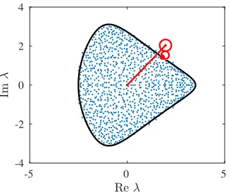
FIG. 4. Polytrochoid curve (black line) bounding the eigen-value spectrum (blue dots) of a sparse regular random di-graphs composed of 3-cycles and 4-cycles, with each node appearing in four of each. In this case the curve is traced by the dot marked on the smaller wheel, which makes three turns around the larger wheel while the larger wheel makes one turn around the orgin, in the opposite direction.
Asymptotically for large ˆd, A(m)(l,dˆ) = dˆl l
ml l−1
= ˆ
dl ml−l+1
ml l
, so that both expressions again match up for
ρ3 ∼ dˆ−1/2. It is worth mentioning that the traces of
M, which can be computed explicitly, relate to asymp-totic spectral statistics in the so-called “trace formulas” which are relevant in random matrix theory [36] as well as in semiclassical physics [37, 38]. These observations lend further support to our conclusion that the cycle structure captures the essential universal features of the eigenvalue distribution beyond the elliptic law.
Polytrochoid spectra.— Starting from Eq. (8), our ap-proach generalizes to matrices with correlations of mul-tiple orders, leading to a boundary curve
zb(ϕ) =e−iϕ+
X
k
ρkei(k−1)ϕ. (19)
The curve described by this equation is an example of the very general polytrochoid family. For the particu-lar case of two competing correlation orders, the curve is described by tracing the path of a point in a wheel rotating around a larger wheel, which itself is rotatingin the opposite direction around the origin. Adding further correlation orders would correspond to the addition of more linked wheels with the same drawing procedure.
Polytrochoid spectral boundaries are also found in di-graphs with mixed cycle lengths, where each vertex con-nects todkk-cycles of weightwk; see [31] for a derivation
in the case of two competing cycle motifs. In the limit of large degrees, we obtain the explicit formula
z ¯ d =e
−iϕ+d 1
w1 ¯ d
k1
ei(k1−1)ϕ+d2 w2
¯ d
k2
ei(k2−1)ϕ,
(20) where ¯d = pd1w12+d2w22. Fig. 4 shows a numerical illustration of this result, which is in excellent agreement
with our derivations for relatively large degrees.
Discussion.— We have shown that high-order correla-tions in the entries of a random matrix give a surpris-ing and even beautiful shape to its eigenvalues, with the boundary given by a hypotrochoid, generalizing the clas-sical result from Girko [7]. Furthermore, we have uncov-ered a remarkable degree of universality of this result by connecting it to the known case of regular graphs with cyclic motifs[19], and studied the relationship between both cases. Our derivations are in excellent agreement with numerical results.
Our results have a simple interpretation in terms of systems theory. A feedback loop is a classical control theory tool to enhance or dampen certain frequencies. A cycle of lengthkwhere the product of the edge weights iswis a feedback loop with delaykand weightw, there-fore a graph with abundance of cycles of length k with positive feedback would resonate at a frequency k1. On the spectral side, the presence of large positive correla-tions of orderk leads to dominant eigenvalues (or poles, in control theory terms) with phases 2πjk forj < k.
This interpretation can also be used in the other di-rection. Matrices and graphs are useful models to repre-sent the interactions between elements, and our results show that random matrix theory can account for intri-cate multi-element interactions. That is, the stability and resonance properties of complex systems with inter-connected feedback loops can be studied by converting the loops into graph cycles and then applying our re-sults in random matrix theory. For example, designing large networked systems such as the Internet or power grids is a challenging problem due to the amount of feed-back loops present [39, 40]. Likewise, biological regula-tory systems [41–43] include many intertwined feedback loops that render their analysis difficult. In all those ex-amples, their stability and dynamical properties can be studied through the spectrum of their adjacency matrix, which can be difficult to estimate. However, finding fre-quent cycles and their corresponding delays is typically easier [44–46], meaning that we can leverage the sim-plicity of finding cycles to obtain rigorous results on the stability of those systems. We hope that the techniques and results presented here may inspire new developments in these fields.
[image:4.612.90.254.58.195.2]sub-graphs implies that there are components dominated by either positive or negative feedback, and thus the effec-tive medium approximation does not hold.
This work was supported by the Royal Society (TR) and EPSRC (HS) via grant EP/P010180/1. The authors are grateful to Izaak Neri for highlighting important prior work on sparse networks with cycles.
∗
†
‡
[1] G. W. Anderson, A. Guionnet, and O. Zeitouni, An Introduction to Random Matrices, Cambridge Studies in Advanced Mathematics (Cambridge University Press, 2009).
[2] A. M. Tulino and S. Verd´u, Found. Trends Commun. Inf. Theory 1, 1 (2004).
[3] T. Guhr, A. M¨uller-Groeling, and H. A. Weidenm¨uller, Phys. Rep.299, 189 (1998).
[4] R. M. May, Nature238, 413 (1972).
[5] S. Allesina and S. Tang, Nature483, 205 (2012). [6] B. Rosenow, inAPS March Meeting Abstracts (2000) p.
P5.004.
[7] V. Girko, Theory Probab. Appl.30, 677 (1986). [8] T. Tao, V. Vu, and M. Krishnapur, Ann. Probab. 38,
2023 (2010).
[9] F. G¨otze, A. Naumov, and A. Tikhomirov, Random Ma-trices: Theory and Applications4, 1550006 (2015). [10] H. H. Nguyen and S. ORourke, International
Mathemat-ics Research Notices2015, 7620 (2014).
[11] G. Marinello and M. P. Pato, Journal of Physics A: Math-ematical and Theoretical51, 375003 (2018).
[12] N. Alexeev and A. Tikhomirov, Journal of Theoretical Probability30, 1170 (2017).
[13] P. V. Aceituno, Y. Gang, and Y.-Y. Liu, arXiv preprint arXiv:1707.02469 (2017).
[14] P. Elbau and G. Felder, Commun. Math. Phys.259, 433 (2005).
[15] P. M. Bleher and A. B. Kuijlaars, Advances in Mathe-matics230, 1272 (2012).
[16] J. Grilli, T. Rogers, and S. Allesina, Nat. Commun.7, 12031 (2016).
[17] T. Rogers, J. Math. Phys.51, 093304 (2010).
[18] C. Bordenave, Electron. Commun. Probab. 16, 104 (2011).
[19] F. L. Metz, I. Neri, and D. Boll´e, Phys. Rev. E 84, 055101(R) (2011).
[20] D. Boll´e, F. L. Metz, and I. Neri, in Spectral analy-sis, differential equations and mathematical physics: a Festschrift in honor of Fritz Gesztesy’s 60th birthday, edited by H. Holden, B. Simon, and G. Teschl (American Mathematical Society, 2013) pp. 35–58.
[21] F. L. Metz, I. Neri, and T. Rogers, Journal of Physics A: Mathematical and Theoretical (2019), (accepted manuscript online).
[22] J. M. Levine, J. Bascompte, P. B. Adler, and S. Allesina, Nature546, 56 (2017).
[23] X. Guo and J. Q. Boedicker, PLOS Comput. Biol. 12, e1005079 (2016).
[24] M.-H. Wang, C. Fiocchi, X. Zhu, S. Ripke, M. I. Kamboh, N. Rebert, R. H. Duerr, and J.-P. Achkar, Hum. Genet. 133, 547 (2014).
[25] T. J. Sejnowski, inAIP Conference Proceedings, Vol. 151 (AIP, 1986) pp. 398–403.
[26] L. Personnaz, I. Guyon, and G. Dreyfus, EPL 4, 863 (1987).
[27] J. Doyle and G. Stein, IEEE Trans. Automat. Contr.26, 4 (1981).
[28] See, for example, US patent 3037488A “Rotary hydraulic motor”, George M Barrett, (1962).
[29] J. Feinberg and A. Zee, Nucl. Phys. B501, 643 (1997). [30] R. A. Janik, W. N¨orenberg, M. A. Nowak, G. Papp, and
I. Zahed, Phys. Rev. E60, 2699 (1999).
[31] See the Supplementary Material at URL *** for details on the matrix generation algorithm, background on the elliptic law and the cavity method, the limiting behaviour of digraphs with a high degree, and the derivation of the spectral density for graphs with two competing cycle motifs. This includes Refs. [47–49].
[32] G. Semerjian and L. F. Cugliandolo, J. Phys. A35, 4837 (2002).
[33] G. Biroli and R. Monasson, J. Phys. A32, L255 (1999). [34] T. Rogers and I. P. Castillo, Phys. Rev. E 79, 012101
(2009).
[35] S. N. Dorogovtsev, A. V. Goltsev, J. F. F. Mendes, and A. N. Samukhin, Phys. Rev. E68, 046109 (2003). [36] F. Haake, M. Kus, H.-J. Sommers, H. Schomerus, and
K. Zyczkowski, J. Phys. A29, 3641 (1996).
[37] F. Haake,Quantum signatures of chaos, Vol. 54 (Springer Science & Business Media, 2013).
[38] M. C. Gutzwiller,Chaos in classical and quantum me-chanics, Vol. 1 (Springer Science & Business Media, 2013).
[39] P. Fairley, IEEE Spectr.41, 22 (2004).
[40] S. H. Low, F. Paganini, and J. C. Doyle, IEEE Contr. Syst. Mag.22, 28 (2002).
[41] R. Thomas, D. Thieffry, and M. Kaufman, Bull. Math. Biol.57, 247 (1995).
[42] A. Becskei and L. Serrano, Nature405, 590 (2000). [43] M. Csete and J. Doyle, Trends Biotechnol. 22, 446
(2004).
[44] R. Milo, S. Shen-Orr, S. Itzkovitz, N. Kashtan, D. Chklovskii, and U. Alon, Science298, 824 (2002). [45] S. S. Shen-Orr, R. Milo, S. Mangan, and U. Alon, Nat.
Genet.31, 64 (2002).
[46] F. A. L´opez, P. Barucca, M. Fekom, and A. C. C. Coolen, J. Phys. A51, 085101 (2018).
[47] J. T. Chalker and B. Mehlig, Phys. Rev. Lett.81, 3367 (1998).
[48] H. Schomerus, K. M. Frahm, M. Patra, and C. W. J. Beenakker, Physica A278, 469 (2000).