Optimizing Sparse Matrix Vector Multiplications on An ARMv8 based Many Core Architecture

ARMv8-based Many-Core Architecture

Abstract. Sparse matrix-vector multiplications (SpMV) are common in scientific and HPC applications but are hard to be optimized. While the ARMv8-based processor IP is emerging as an alternative to the tradi-tional HPC processor design, there is little study on SpMV performance on such new many-cores. To design efficient HPC software and hardware, we need to understand SpMV behavior. This work develops a quantita-tive approach to characterize SpMV performance on a recent ARMv8-based many-core architecture, Phytium FT-2000Plus (FTP). We perform extensive experiments involved over 9,500 distinct profiling runs on 956 sparse datasets and five mainstream sparse matrix storage formats, and compare FTP against the Intel Knights Landing many-core. We experi-mentally show that picking the optimal sparse matrix storage format and parameters is non-trivial as the correct decision requires expert knowl-edge of the input matrix and the hardware. We address the problem by proposing a machine learning based model that predicts the best storage format and parameters using input matrix features. The model automat-ically specializes to the many-core architectures we considered. Experi-mental results show that our approach achieves on average 93% of the best-available performance without incurring runtime profiling overhead. Keywords: SpMV·Sparse matrix format·Many-Core·Performance .

1

Introduction

The sparse matrix-vector multiplication (SpMV)1_{is one of the most common} op-erations in scientific and high-performance-computing (HPC) applications [18]. While SpMV is often responsible for the application performance bottleneck, it is notoriously difficult to be optimized. This is due to a number of inherent is-sues arising from the computation kernel, the matrix storage format, the sparsity pattern of the input matrix, and the complexity of parallel hardware [10, 11].

Numerous sparse matrix storage formats have been proposed [1, 6, 7, 10, 14, 20], all aiming to reduce the memory footprint by only storing a fraction of the elements of the target matrix. While there is an extensive body of work on optimizing SpMV on SMP and multi-core architectures [10, 11], there is little work on investigating SpMV performance on ARM-based many-core architec-tures. Given that ARM-based processor IP is emerging as an alternative for HPC processor architecture [8, 19, 22], it is crucial to understand how well dif-ferent sparse matrix storage formats perform on such architectures and what affects the resulting performance. Understanding this can not only help software developers to write better code for the next-generation HPC systems, but also provide useful insights for hardware architects to design more efficient hardware for this important application domain.

1

This paper studies the SpMV performance on the latest ARMv8-based Phytium FT-2000Plus (FTP) [16, 22]. This architecture integrates over 60 processor cores to offer a powerful computation capability, making it attractive for the next-generation HPC systems. We conduct a large-scale evaluation involved over 9,500 profiling runs performed on 956 representative sparse datasets and consider five widely-used sparse matrix representations: CSR [20], CSR5 [10], ELL [6], SELL [7, 14], and HYB [1]. We also compare SpMV performance on FTP against the Intel Knights Landing (KNL) multi-core that has been deployed in many HPC systems. This comparison provides insights on whether an ARMv8-based many-core requires a different optimization strategy for SpMV computation.

We demonstrate that although there is significant gain for choosing the right sparse matrix storage format and parameters, mistakes can seriously hurt the performance. We then investigate what cause the performance disparity. Our data show that picking the optimal storage format and parameters requires ex-pert knowledge of the underlying hardware and the input matrix. To help devel-opers to choose the right storage format, we employ machine learning to develop a predictive model. Our model is trainedofflineusing a set of training examples. The inputs to the model are static features extracted from the input matrix. The trained model is then used atruntime to choose the optimal storage format for anyunseensparse matrix. Experimental results show that our approach is highly effective in choosing the sparse matrix storage format, delivering on average over 90% of the best-available performance on FTP and KNL.

In summary this paper makes the following contributions:

– We provide the first extensive characterization of SpMV performance on FTP, an emerging ARMv8-based many-core architecture for HPC;

– We reveal how the storage format parameters and hardware architecture differences affect the SpMV performance on FTP and KNL;

– We develop a machine learning technique to predict the best sparse matrix storage format, which is portable across many-core architectures.

2

Background and Experimental Setup

In this section, we describe the sparse matrix storage formats considered in this work and our experimental setup.

2.1 Sparse Matrix Storage Formats

We consider five mainstream sparse matrix storage formats, described as follows.

CSR.Thecompressed sparse row (CSR) format explicitly stores column indices and nonzeros in arrays indices and data, respectively. It uses a vector ptr, which points to row starts in indices and data, to query matrix values. The length ofptrisn row+1, where the last item is the total number of the nonzero elements of the matrix.

CSR5. The CSR5 format aims to obtain a good load balance for matrix value

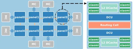
Fig. 1.A high-level overview of the FTP architecture.

ELL. For an M ×N matrix with a maximum number of K nonzero elements per row, TheELLPACK-Itpack(ELL) format stores the sparse matrix in a dense

M ×K array. If there are fewer than K elements in a row, the row is padded with zeros. ELL uses an integer companion array,indices, to store the column indices of the each nonzero element. This scheme may be inefficient if many rows of the target matrix have fewer thanK elements.

SELL. Sliced ELL (SELL) is an extension to the ELL format by partitioning

the input matrix into strips of Cadjacent rows [14]. Each strip is stored in the ELL format but the number of nonzero elements of each strip may be different. Because the number of stored elements in each row is no longer determined by the maximum of nonzero elements of a row but by the “longest row” in this strip of rows, some of the slices may require less storage space compared to ELL. SELL-C-σimproves the vanilla SELL by adding row sorting such that rows with similar number of nonzero elements are grouped in one block [7]. To trade-off the cost of sorting against the acceleration of the SpMV, rows are not sorted globally but within σ consecutive rows. In this work, we use SELL-C-σ and refers it as SELL to aid readability thereafter.

HYB. The HYB format is a combination of ELL and the simple COO format which explicitly stores indices of the row, column, and values of nonzero ele-ments [1]. For each matrix row, HYB storesK nonzero elements using the ELL format and the remaining elements in COO.

2.2 Evaluation Setup

Hardware Platforms. As depicted in Figure 1, FTP integrates 64 ARMv8

Systems Software. We run a customized Linux OS with Linux Kernel v4.4 and v3.10 on FTP and KNL respectively. For compilation, we use gcc v6.4.0 on FTP and Intel icc v17.0.4 on KNL with the “-O3” compiler option. We use the OpenMP threading model, using 64 threads on FTP and 72 threads on KNL.

Datasets. We use 956 square matrices (with a total size of 90 GB) from the

SuiteSparse matrix collection [3]. The number of nonzero elements of the matri-ces ranges from 100K to 20M. The dataset includes both regular and irregular matrices, covering domains from scientific computing to social networks.

3

SpMV Performance Analysis

3.1 Roadmap

Recall that our goal is to understand how different sparse matrix storage for-mats perform on FTP. In addition to the sparse matrix storage format, memory allocation and code optimization can also affect the SpMV performance. To iso-late the problem, we need to find out the optimal memory allocation and code optimization scheme. For memory allocation, we investigate Non-Uniform Mem-ory Access (NUMA) bindings. For code optimization, we look at vectorization because it is an important optimization opportunity for matrix multiplications. We then study the impact of the sparse matrix storage format by using the best-found strategy of NUMA memory allocation and code vectorization.

3.2 The Impact of NUMA Bindings

FTP exposes eight NUMA nodes where a group of eight cores are directly con-nected to a local memory module. Indirect access to remote memory modules is possible but 1.5x slower than accessing the local module. Here we use the Linux NUMA utility, numactl, to allocate the required data buffers from the local memory module for an OpenMP thread that performs SpMV computation.

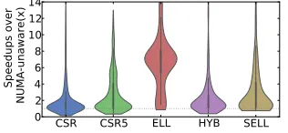
As can be seen from Figure 2, NUMA-aware memory allocation significantly outperforms the non-NUMA-aware counterpart, giving an average speedup rang-ing from 1.5x to 6x across five storage formats. As such, we enable static NUMA bindings on FTP. We also observe that the ELL format consumes the largest memory buffers among the five storage formats, and thus we can achieve the maximum speedup with manual NUMA bindings.

3.3 The Impact of Code Vectorization

CSR CSR5 ELL HYB SELL 02

4 6 8 1012 14

Speedups over

NUMA-unaware(x)

Fig. 2.The violin diagram shows the speedup distribution of NUMA-aware memory allocation on FTP. The thick black line shows where 50% of the data locates.

CSR CSR5 ELL HYB SELL

01

2 3 4 5 6 7 8

Speedups KNL vs FTP (x)

(a) KNL over FTP

C S R C S R 5 E L L S E L L H Y B

0

1 0 2 0 3 0 4 0 5 0 6 0

%

o

f b

ei

ng

o

pt

im

al F T P K N L

(b) Optimal storage format distribution

Fig. 3.Sub-figure (a) shows the speedups of KNL over FTP and sub-figure (b) suggests the optimal storage format changes from one architecture to the other.

not support thegatheroperation which is essential for accessing elements from different locations of a vector. Our findings suggest that future ARMv8-based many-core designs perhaps should support thegatheroperation to achieve good vectorization performance. For the remaining experiments in this work, we use the manually vectorized code on KNL and the non-vectorized code on FTP.

3.4 The Impact of Hardware Architecture Differences

Figure 3(a) compares the performance by running the same kernel on KNL over FTP. KNL outperforms FTP by delivering, on average, at least 1.3x speedup (up to 2.1x) across the five storage formats. The performance advantage of KNL primarily comes from its Multi-Channel DRAM (MCDRAM) which provides more than 6x bandwidth over the traditional DDR memory. MCDRAM signif-icantly reduces the memory access latency once the data is loaded into it. The performance benefit of KNL also comes from the better support of code vec-torization as mentioned in Section 3.3. On the other hand, we observe that on some matrices, especially when the matrix size is small, FTP delivers better performance over FTP. This is largely due to the larger L2 data cache on FTP and a more efficient coherence protocol. Overall, our results suggest that a fast memory hierarchy is essential for obtaining good SpMV performance.

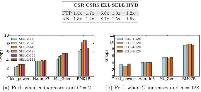
Table 1.The average slowdown (x) over the optimal when using a fixed storage format.

CSR CSR5 ELL SELL HYB

FTP 1.5x 1.7x 6.6x 1.3x 1.2x

KNL 1.3x 1.4x 8.7x 1.5x 1.6x

kkt_power Hamrle3 ML_Geer RM07R 0 2 4 6 8 10 Gflops SELL-2-16 SELL-2-32 SELL-2-64 SELL-2-128 SELL-2-256 SELL-2-512

(a) Perf. whenσincreases andC= 2

kkt_power Hamrle3 ML_Geer RM07R 0 2 4 6 8 1012 Gflops SELL-1-128 SELL-2-128 SELL-4-128 SELL-8-128

(b) Perf. whenCincreases andσ= 128

Fig. 4.The impact ofσand C on SpMV performance.

msdoor nd12k pkustk10 oilpan

7 8 9 10 11 12 Gflops histogram traditional

(a) Performance with different strategies

0 10 20 30 40 50 60 70 80 5.5 6.0 6.5 7.0 7.5 8.0 8.5 9.0 Gflops histogram traditional A HYB ELL CSR

(b) Performance when K increases Fig. 5.How the change ofKof HYB affects the SpMV performance.

half of the matrices on KNL, it should only be used for 10% of the matrices on FTP. This diagram suggests that the choice of the storage format depends on the underlying hardware. Table 1 gives the average slowdowns when using a fixed format across all test cases over the optimal one. The slowdown has a negative correlation with how often a given format being optimal. Using a fixed format can miss significant optimization opportunities with up to 6.6x and 8.7x slowdowns on FTP and KNL respectively. This experiment shows that there is no “one-fits-for-all” storage format across matrices and architectures. As such we need to have an adaptive scheme to help developers to choose the optimal sparse matrix format. In Section 4, we describe how to develop such an approach using machine learning.

3.5 The Impact of Storage Format Parameters

We now consider the impact of choosing storage format parameters. Among the five storage formats considered in this work, SELL has two tuning parameters,C

SELL We choose four matrices, RM07R, kkt power, Hamrle3, andML Geer, to evaluate how different values ofCandσaffect the performance of SELL. These four matrices are chosen because they represent distinct matrix characteristics. Figure 4(a) shows the resulting performance as σ increases when we fix C

to 2 (which matches the double-precision register width of FTP). We observe improved performance for all matrices when using a largerσ, which in turns leads to less padding operations (see Section 2.1), but the performance improvement reaches a plateau when σis set to 128. This is because a largerσalso means a bigger sorting scope, which is more likely to increase the load imbalance.

Figure 4(b) shows how the change of C affects the performance. In this experiment, we fixσto the overall optimal value of 128. Here, we observe little change in performance with differentCvalues. This is because while a largerC

enables more aggressive loop unrolling (which can improve performance), it also incurs more padding operations which can eclipse the benefit of loop unrolling.

HYB Recall that HYB stores K nonzero elements in ELL and the rest in COO. Thus, the choice ofK can have an impact of the SpMV performance. In this experiment, we compare two algorithms for choosingK: an average based algorithm [2] and a “histogram” based scheme [1]. This evaluation is performed on four matrices listed in Figure 5(a) to keep the experiments manageable. Note that these matrices are different from those used to study SELL, because these are the matrices where HYB is the optimal choice.

As can be seen from Figure 5(a), the “histogram” based algorithm delivers, on average, 10% performance improvement over its counterpart. Figure 5(b) shows how the performance onmsdoorchanges whenKis increased from 1 to 80. HYB could be a good storage format for the considered matrices, but this requires ones to choose the correctK value. A wrongKvalue can lead to significantly worse performance, e.g., the point marked with labelA in Figure 5(b). This example shows how important it is to choose the right parameter setting.

4

Predictive Modeling for Storage Format Selection

We develop an automatic machine learning approach to automatically choose the correct sparse matrix storage format. Our approach takes a new, unseen

sparse matrix and is able to predict the optimal or near optimal sparse matrix representation for a given architecture. To demonstrate the portability of our approach, we train and evaluate a predictive model on FTP and KNL.

Our model for predicting the best sparse matrix storage format is a decision-tree-based random forests model [4]. We have evaluated other alternative tech-niques, including regression, Naive Bayes and K-Nearest neighbour (see also Sec-tion 5.2). We chose the decision tree model because it gives the best performance and can be easily interpreted compared to other black-box models.

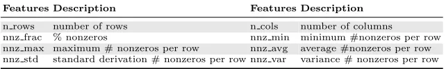
Table 2.The features used in our model.

Features Description Features Description

n rows number of rows n cols number of columns

nnz frac % nonzeros nnz min minimum #nonzeros per row nnz max maximum # nonzeros per row nnz avg average #nonzeros per row nnz std standard derivation # nonzeros per row nnz var variance # nonzeros per row

4.1 Training the Predictor

To train a predictor we first need to find the best sparse matrix storage format for each of our training examples, and extract features. We then use this set of data and classification labels to train our predictor model.

Generating Training Data. We use the standard five-fold-cross validation

for training. Specifically, we select, from the SuiteSparse matrix collection, 20% samples for testing and then use 80% samples (i.e., 756 matrices) for training. We execute SpMV using each of the targeting sparse matrix storage formats. We run each training setting several times until the gap of the upper and lower confidence bounds is smaller than 5% under a 95% confidence interval setting. We then record the best-performing storage format for each training sample on our target hardware platform. Finally, we extract the values of our selected set of features from each matrix.

Building The Model. The optimal matrix storage labels, along with their

corresponding feature set, are passed to our supervised learning algorithm. The learning algorithm tries to find a correlation between the feature values and optimal representation labels. The output of our learning algorithm is a version of our random forests model. Since training is performed off-line and only need to be carried out once for a given architecture, this is aone-off cost.

Total Training Time. The total training time of our model is comprised of

two parts: gathering the training data, and then building the model. Gathering the training data consumes most of the total training time, in this paper it took around 3 days for the FTP and KNL platforms. In comparison actually building the model took a negligible amount of time, less than 10 ms.

4.2 Features

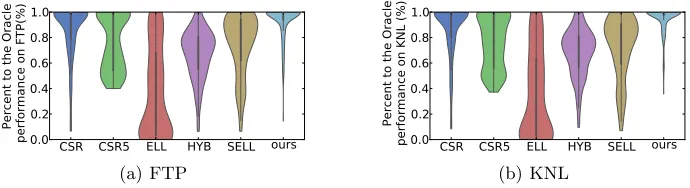
CSR CSR5 ELL HYB SELL ours 0.0

0.2 0.4 0.6 0.8 1.0

Percent to the Oracle

performance on FTP(%)

(a) FTP

CSR CSR5 ELL HYB SELL ours 0.0

0.2 0.4 0.6 0.8 1.0

Percent to the Oracle

performance on KNL (%)

(b) KNL

Fig. 6.The predicted performance of SpMV on FTP and KNL. We show the achieved performance with respect to the best available performance across sparse formats.

its importance. We record the minimum and maximum values of each feature in the training dataset, and use these to scale the corresponding features for an unseen input during deployment.

4.3 Runtime Deployment

The trained model is encapsulated in a runtime library. We provide an API to extract matrix features and a tool to perform matrix format transformation. For a given matrix, our tool automatically translates it to the five targeted storage formats of parameter settings. The transformation is performed offline and does not incur runtime overhead. During runtime, the off-line trained model predicts the optimal storage format and parameters to use, and the library automatically selects the offline generated format to run on the target architecture.

5

Predictive Modeling Evaluation

5.1 Overall Performance

As described in Section 4.1, we use cross-validation to train and test our pre-dictive model to make sure the model is evaluated on new, unseen inputs. We repeat the cross-validation process multiple times to ensure all matrices in our dataset are tested at least once.

Figure 6 shows that our predictor achieves, on average, 93% and 95% of the best available SpMV performance (found through exhaustive search) on FTP and KNL respectively. We also note that our predictor outperforms a strategy that uses only the single overall-best format on each platform, i.e., SELL or HYB on FTP and CSR on KNL (see Table 1). This experiment shows that our predictor is highly effective in choosing the right sparse matrix representation.

5.2 Alternative Modeling Techniques

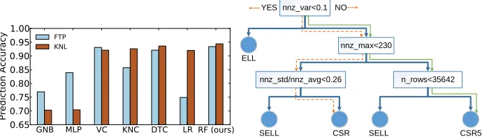
GNB MLP VC KNC DTC LR RF (ours)

0.65

0.700.75

0.800.85

0.900.95

1.00

Prediction Accuracy

FTP KNL

Fig. 7.Compare to alternative classifiers.

nnz_var<0.1

nnz_max<230

ELL

nnz_std/nnz_avg<0.26 n_rows<35642

SELL CSR SELL CSR5

YES NO

Fig. 8.How two unseen matrices follow the different paths of a learned tree.

bayes (GNB), multilayer perception (MLP), soft voting/majority rule Classifi-cation (VC), k-Nearest Neighbor (KNC, k=1), logistic regression (LR), decision tree classification (DCT). Thanks to the high-quality features, all classifiers are highly accurate in choosing sparse matrix representation. We choose RF because its accuracy is comparable to alternative techniques.

5.3 Analysis of The Predictive Model

One of our motivations for using a decision-tree-based random forests model is that this modeling technique is interpretable. This means that we can gain insights of why a certain storage format is chosen.

Figure 8 shows one of the decision trees in our random forests model on FTP. The learning algorithm automatically places the most relevant features at the root level and determines the architecture-dependent threshold for each node. All this is done automatically without the need of expert intervention.

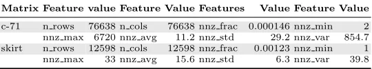
Table 3 lists the feature values extracted from two distinct matrices, c-71

and skirt. To choose a storage format, we follow the decision tree depicted in

Figure 8. At the root of the tree, we look at the value for the nnz var. This feature uses the variation (i.e., dispersion) for the number of nonezero elements among rows to measure the matrix regularity. The values are far above the threshold, suggesting that the nonzero elements are not evenly distributed in both matrices. We thus go to the right subtree and reach the second level of the tree. This node looks atnnz max. The feature value of c-71 is larger than the threshold and therefore the right branch is taken, but forskirt we choose the left branch. The metric of nnz max counts the largest number of nonzero elements within a row. A large value in the feature suggests that the longest row is likely to cause load imbalance. In such a case, storage formats like CSR5 and SELL may be a good fit because they are designed to avoid load imbalance. At the second-last level of the tree, we look at nnz rows andnnz std / nnz avg

Table 3.Feature values of matrixc-71andskirt. Matrix Feature value Feature Value Features Value Feature Value

c-71 n rows 76638 n cols 76638 nnz frac 0.000146 nnz min 2 nnz max 6720 nnz avg 11.2 nnz std 29.2 nnz var 854.7 skirt n rows 12598 n cols 12598 nnz frac 0.00123 nnz min 1 nnz max 33 nnz avg 15.6 nnz std 6.3 nnz var 39.8

6

Related Work

A large body of work has been conducted in the past to study SpMV performance on parallel systems [13, 17, 20]. However, our work is the first comprehensive study for SpMV performance on an ARMv8-based many-core. Our work fills the gap by providing an in-depth performance analysis on two emerging many-core architectures (KNL and FTP). The insights will be useful for designing more efficient parallel HPC software and hardware in the future.

Efforts have been made in designing new storage formats for various parallel processor architectures including SIMD CPUs and SIMT GPUs [1, 5, 10, 11, 12, 20, 21]. However, how well these existing sparse matrix formats perform on ARM-based many-cores remains an open problem. Our work attempts to answer this question by providing comprehensive analysis and new insights.

It is shown that there is no universally optimal sparse matrix storage for-mat [23]. Thus, it is important to choose the right forfor-mat according to the right input matrix features to achieve good SpMV performance. Prior work has devel-oped methods to choose a sparse matrix storage format [9, 18], but no work has targeted an ARM-based many-core architecture. Recently, Zhao et al. employ deep learning to automatically extract important features from the input matri-ces to help to build a predictive model [23]. Their approach of feature extraction is thus orthogonal to our machine learning based approach.

7

Conclusion

[1] Bell, N., Garland, M.: Implementing sparse matrix-vector multiplication on throughput-oriented processors. In: SC (2009)

[2] Chen, S., Fang, J., Chen, D., Xu, C., Wang, Z.: Adaptive optimization of sparse matrix-vector multiplication on emerging many-core architectures. In: HPCC (2018)

[3] Davis, T.A., Hu, Y.: The university of florida sparse matrix collection. ACM Trans. Math. Softw. (2011)

[4] Ho, T.K.: Random decision forests. In: ICDAR. pp. 278–282 (1995)

[5] Im, E., Yelick, K.A., Vuduc, R.W.: Sparsity: Optimization framework for sparse matrix kernels. IJHPCA (2004)

[6] Kincaid, D., et al.: Itpackv 2d user’s guide. Tech. rep., Center for Numerical Analysis, Texas Univ., Austin, TX (USA) (1989)

[7] Kreutzer, M., Hager, G., Wellein, G., Fehske, H., Bishop, A.R.: A unified sparse matrix data format for efficient general sparse matrix-vector multiplication on modern processors with wide SIMD units. SIAM J. Scientific Computing (2014) [8] Laurenzano, M.A., Tiwari, A., Cauble-Chantrenne, A., Jundt, A., Jr., W.A.W.,

Campbell, R.L., Carrington, L.: Characterization and bottleneck analysis of a 64-bit armv8 platform. In: ISPASS (2016)

[9] Li, J., Tan, G., Chen, M., Sun, N.: SMAT: an input adaptive auto-tuner for sparse matrix-vector multiplication. In: PLDI (2013)

[10] Liu, W., Vinter, B.: CSR5: an efficient storage format for cross-platform sparse matrix-vector multiplication. In: ICS (2015)

[11] Liu, X., Smelyanskiy, M., Chow, E., Dubey, P.: Efficient sparse matrix-vector multiplication on x86-based many-core processors. In: ICS (2013)

[12] Maggioni, M., Berger-Wolf, T.Y.: An architecture-aware technique for optimizing sparse matrix-vector multiplication on gpus. In: ICCS (2013)

[13] Mellor-Crummey, J.M., Garvin, J.: Optimizing sparse matrix - vector product computations using unroll and jam. IJHPCA (2004)

[14] Monakov, A., Lokhmotov, A., Avetisyan, A.: Automatically tuning sparse matrix-vector multiplication for GPU architectures. In: HIPEAC (2010)

[15] Pedregosa, F., et al.: Scikit-learn: Machine learning in Python. Journal of Machine Learning Research (2011)

[16] Phytium Technology Co. Ltd.: FT-2000 (February 2017), http://www.phytium. com.cn/Product/detail?language=1&product_id=7

[17] Pinar, A., Heath, M.T.: Improving performance of sparse matrix-vector multipli-cation. In: SC (1999)

[18] Sedaghati, N., Mu, T., Pouchet, L., Parthasarathy, S., Sadayappan, P.: Automatic selection of sparse matrix representation on gpus. In: ICS (2015)

[19] Stephens, N.: Armv8-a next-generation vector architecture for HPC. In: 2016 IEEE Hot Chips 28 Symposium (HCS). pp. 1–31 (2016)

[20] Williams, S., Oliker, L., Vuduc, R.W., Shalf, J., Yelick, K.A., Demmel, J.: Opti-mization of sparse matrix-vector multiplication on emerging multicore platforms. In: SC (2007)

[21] Williams, S., Oliker, L., Vuduc, R.W., Shalf, J., Yelick, K.A., Demmel, J.: Opti-mization of sparse matrix-vector multiplication on emerging multicore platforms. Parallel Computing (2009)

[22] Zhang, C.: Mars: A 64-core armv8 processor. In: HotChips (2015)