Estimating Ocean Chlorophyll Using the Penalized Three Dimensional (3D) Blending Technique

(1)

ISSN Online: 2161-7392 ISSN Print: 2161-7384

DOI: 10.4236/ojms.2018.83021 Jul. 18, 2018 386 Open Journal of Marine Science

Estimating Ocean Chlorophyll Using the

Penalized Three Dimensional (3D)

Blending Technique

Mathias A. Onabid

1

, Simon Wood

2

1_{Department of Mathematics-Computer Science, Faculty of Sciences, Dschang, University of Dschang, West Region, Cameroon} 2_{Department of Mathematical Sciences, University of Bath, Bath, UK}

Abstract

The Thin Plate Regression Spline (TPRS) was introduced as a means of smoothing off the differences between the satellite and in-situ observations during the two dimensional (2D) blending process in an attempt to calibrate ocean chlorophyll. The result was a remarkable improvement on the predic-tive capabilities of the penalized model making use of the satellite observa-tion. In addition, the blending process has been extended to three dimen-sions (3D) since it is believed that most physical systems exist in the three dimensions (3D). In this article, an attempt to obtain more reliable and ac-curate predictions of ocean chlorophyll by extending the penalization process to three dimensional (3D) blending is presented. Penalty matrices were computed using the integrated least squares (ILS) and integrated squared derivative (ISD). Results obtained using the integrated least squares were not encouraging, but those obtained using the integrated squared de-rivative showed a reasonable improvement in predicting ocean chlorophyll especially where the validation datum was surrounded by available data from the satellite data set, however, the process appeared computationally expensive and the results matched the other methods on a general scale. In both case, the procedure for implementing the penalization process in three dimensional blending when penalty matrices were calculated using the two techniques has been well established and can be used in any similar three dimensional problem when it becomes necessary.

Keywords

Integrated Least Squares, Integrated Squared Derivative, Basis Function, Penalty Matrix, Penalized Model, In-Situ, Satellite

How to cite this paper: Onabid, M.A. and Wood, S. (2018) Estimating Ocean Chlo-rophyll Using the Penalized Three Dimen-sional (3D) Blending Technique. Open Journal of Marine Science, 8, 386-394.

https://doi.org/10.4236/ojms.2018.83021

Received: June 4, 2018 Accepted: July 15, 2018 Published: July 18, 2018

http://creativecommons.org/licenses/by/4.0/

(2)

DOI: 10.4236/ojms.2018.83021 387 Open Journal of Marine Science

1. Introduction

As stated clearly by [1], most physical systems exist in three space dimensions and that representation in one or two space dimensions entails a lot of approxi-mation. The importance of the ocean environment and its constituent elements to the society as a whole and to decision makers in particular cannot be over-emphasized especially when it concerns marine activities such as fishing and its effect on society. It is therefore not only important to study the ocean environ-ment, but to study it accurately. Aquatic life and production revolve about the distribution and biomass of, phytoplankton, which are found in the upper layer of the ocean. Thus, to better understand the ocean food chain, it is necessary to track their existence and population in this environment. [2] outlined a tech-nique on how to calibrate this phytoplankton in terms of their photosynthetic pigment content, chlorophyll, which is endemic across all taxonomic groups of algae. In fact, [3] and [4] emphasized that a better way to estimate primary prod-uctivity in the ocean is by determining the concentration of ocean chlorophyll.

The blending technique used by [5] in Sea Surface Temperature (SST) analysis was introduced in the calibration of ocean chlorophyll by [6]. In this technique, the in situ observations are assumed to be correct and inserted into the final blended field without modification. The technique acknowledges the fact that the in situ values may be noisy but fails to provide a means of treating it. Some of the problems they encountered were analyzed and solutions proposed by [7]

with the Corrector Factor technique producing better results. In an attempt to improve on the predicting potentials of the blending technique, [8] extended the blending to three dimensions (3D). This was in conformity with the assertion of

[1]. The resulting model did not only provide better predictions of the in situ

observations in areas where bottle samples could not be obtained but also pro-vide a smooth variation of the distribution of ocean chlorophyll throughout the year. In addition, it was computationally efficient since data set that could have been otherwise run severally would be run only once.

1.1. Research Problem

Under normal circumstances, one would expect in situ to have a smooth rela-tionship with satellite data in areas where observations are available from both data sets. This expectation is not met, indicating that some unknown factors may be affecting this relationship. Apart from the drawbacks of the algorithm for converting reflectance data to ocean chlorophyll concentration by not taking in-to account weather conditions and water characteristics, which in turn vary with ocean depth, other factors like seasons of the year, day and location of sample collection could also have an influence on this relationship. In addition, [2]

(3)

DOI: 10.4236/ojms.2018.83021 388 Open Journal of Marine Science correlate well. There is therefore a need to search for methods of predicting reli-able ocean chlorophyll concentrations under such circumstances.

1.2. Research Objective

The lack of a smooth relationship between satellite and in situ field could be caused by the noisiness of both data sets as stated by [7]. In an attempt to treat the noisiness of the in situ observations, [2] suggested a nonparametric statistical approach using the penalized regression splines of [9]. Here, remote sensed chlorophyll data were calibrated by modeling in situ data as a smooth function of satellite observations, time of the year and ocean depth. In this approach, the difficulty was to find a means of scaling the parameters relative to one another since they were to be used as parameters of a single smooth function. Another attempt to treat the noisiness of the data set was suggested by [10] in which pe-nalization was implemented on the two dimensional blending technique. Results obtained showed a remarkable improvement on the prediction of ocean chloro-phyll from the satellite data.

This result motivated the main objective of the research, which is to extend the penalization of the blending technique from two dimensions to three dimen-sions (3D) since it is believed that most physical systems when expressed in three dimensions makes them closer to reality. The process of penalization requires smoothing, thus the efficiency of the technique will depend on the choices of the smoothing parameters. The procedure for selecting the smoothing parameter for the three dimensional penalization will follow some of the techniques used by

[10] in case of two dimensions and results obtained by using each of the smoothing parameter shall be compared. In order to apply the penalization pro-cedure, it was necessary to represent the blending process using basis function.

2. Expressing the Three Dimensional Blending Model Using

Basis Function

The extension of smoothing the blending process from two to three-dimensions is very similar to the extension of the blending process itself from two to three dimensions. Hence expressing the three-dimensional blending process in the ba-sis function mode can be done by extending the two dimensional baba-sis function equation of [10] given as

( )

1

, , n ,

blend sat k

k

f x y f x y g x y

=

= +

∑

(1) where gk is the solution to

2 2

2 2 0

g g

x y

∂ ∂

+ =

∂ ∂ , subject to the boundary conditions

{

0, , :x y ii i =1, , , k k+1, , , , , n ∆k x yk k

}

. Extension to three dimensions was

done with the addition of time, averaged over weeks as the third variable. When this is done, Equation (1) can then be written in three dimensions as follows:

(

)

(

)

(

)

1

, , , , , ,

blend sat k

n

k

f x y z f x y z g x y z

=

= +

∑

(4)

DOI: 10.4236/ojms.2018.83021 389 Open Journal of Marine Science where gk is the actual solution to the three dimensional partial differential

eq-uation

2 2 2

2 2 2 0

g g g

x y z

∂ ∂ ∂

+ + =

∂ ∂ ∂

(3) subject to the boundary conditions

{

0, , , :x y z ii i i =1, , , k k+1, , , , , , n ∆k x y zk k k

}

.

Equation (2) can be re-written with each of the gk separately as

(

)

(

)

(

)

1

, , , , n , ,

blend sat k k

k

f x y z f x y z

β

x y z

=

= +

∑

∆

(4) where βk is set to the difference between the in situ and satellite values at

boundary point k and∆k

(

x y z, ,

)

representing the basis is the solution to

2 2 2

2 2 2 0

g g g

x y z

∂ ∂ ∂

+ + =

∂ ∂ ∂

with external boundary points set to zero and the internal boundary points set to zero everywhere except at the kth_{position where it is set to 1.0, that is the}_knot_of the basis. The blending process is performed using this knot as the sole boun-dary point, and the solution obtained is the basis for that knot. The sum of the product of each knot and its basis is added to the satellite field to give the final blended field of the basis function method.

3. Penalizing the Three Dimensional Blending

In order to penalize the three dimensional blending model, it was necessary to represent it in a regression equation form. This can be done using Equation (4) where the term of interest is

(

)

1 k , ,

k n

k x y z

β

=

∆

∑

From the two dimensional regression equations in [9], the three dimensional regression equations can be written in form

(

)

1 , ,

k j j j j j k

j n

Z β x y z ε

=

∑

∆ +

(5)

where βj are unknown parameters to be estimated and ∆j

(

x y zj, ,j j

)

the

ba-sis corresponding to the point j while εk is the error term. This expression has

been shown by [10] to be equal to

(

, ,

)

k j j j j j k

Z =

β

∆ x y z +

ε

And the estimation of the parameters can be done using the nonparametric technique of penalized regression spline. This can be done by solving the pena-lized least squares objective given as

(

)

2

(

)

1

, , , ,

k k k k k k k k k k k

k n

Z

β

x y z

λ β

x y z

=

 − ∆ _ − ∆



∑

(5)

DOI: 10.4236/ojms.2018.83021 390 Open Journal of Marine Science and the smoothing parameter

λ

_{. These, can be obtained from generalized cross}

validation (gcv) and will therefore require the calculation of the collective penal-ty matrix S which penalizes the difference between the satellite and in situ fields. This shall be done by using the procedures of integrated least squares and the integrated squared derivatives. The ridge regression ended up in complete de-coupling in the two dimensional case and thus shall not be tried here.

3.1. Using the Integrated Least Squares

Though this techniques was not successful in the two dimensional case because of the sparseness of data, its description here is to fine out its performance when more information is made available and secondly to provide a means of imple-menting it in three dimensions when it becomes necessary. Thus by using the integrated least squares, a collective penalty in the three dimensions was im-posed on the term

(

)

1 k , ,

k n

k x y z

β

=

∆

∑

By so doing, the penalty term could be written as

(

)

2

, , d d d

x y z x y z δ

 

 

∫∫∫

By evaluating the three dimensional integral, the n × n penalty matrix S was obtained. That is

(

)

2

, , d d d

S=

_∫∫∫

_δ x y z _ x y z

This was approximated by performing pair wise sums in each spatial direction as

(

) (

)

, , , , ,

i j i q q q j q q q

S ≈ ∆

∑

x y z ∆ x y z

by summing over all the grid points

(

x y zq, ,q q

)

. Once this matrix has been

cal-culated, the model fitting process becomes straight forward. That is, given any sequence of smoothing parameters (λ’s), and the selected knots (β’s), models were be fitted to choose the optimum gcv score and optimum trace value.

These was then be used to fit the penalized model. The result obtained here was not encouraging, as predictions from these models were worse than those from the normal three-dimensional blending. This gave way to the examination of penalization using the integrated squared derivative in the three-dimensions.

3.2. Using Integrated Squared Derivative

In the case of the integrated squared derivative, the penalty is calculated based on the derivative of the basis function. This is represented by

2

2 2

d d d _{d d d ,}

d d d

u u u

S x y z

x y z

_ _ _ _ _ _ 

 

= _ _ +_ _ +_ _

   

   

 

∫

(6)

(

) (

)

1

, , , ,

k k k

n

u

β

x y z x y z

=

∑

∆ = ∂

The penalty S will be obtained from evaluation the integral. Therefore the n × n penalty matrix S was obtained by evaluating

2

2 2

T T T

T

T T T

T T

d _{d d d} d _{d d d} d _{d d d}

d d d

d d _{d d d} d d _{d d d} d d _{d d d}

d d d d d d

T T

T

u u u

S x y z x y z x y z

x y z

x y z x y z x y z

x x y y z z

x y z x y z x y z

x x y y z z

β β β β β β

 

   

= _ _ + _ _ + _ _

     

∂ ∂ ∂ ∂ ∂ ∂

= + +

∂ ∂ ∂ ∂ ∂ ∂

= + +

∫

The penalty matrix S is obtained by evaluating

T T T

d dx x x y z d dy y x y z d dz z x y z

∂ ∂ ₊ ∂ ∂ ₊ ∂ ∂

∫

These integrals can be approximated by the sums of product of the differences over all pairs of basis functions to obtain the n × n matrix S. This is then used to calculate the gcv score. The λ corresponding to the minimum gcv score is se-lected as the optimum smoothing parameter which is then used to fit the pena-lized regression model.

4. Validating the Three-Dimensional Blended Fields

The data set used for validation is an extract obtained from the archive main-tained by the National Oceanic and Atmospheric Administration (NOAA) Na-tional Oceanography Data Centre (NODC), comprising observations from 1997 to 2002 averaged over a grid size of 0.75 longitude by 0.75 latitude and using the successive 8-day intervals over the year. This is justified by the fact that this same data set has been used in previous attempts to calibrate ocean chlorophyll and in addition, there is need to compare the performance of previous models and the model herein described.

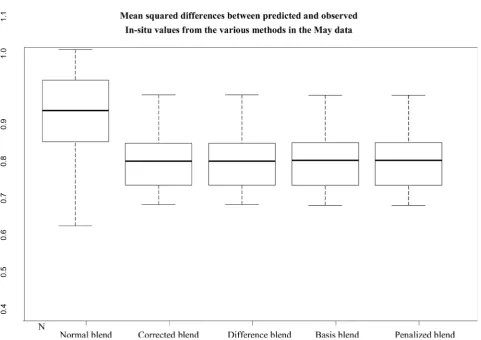
Considering the large number of in situ observations available when looking at the data field in three-dimensions and the large amount of computer memory required running the evaluation of the penalty matrix, only data for the month of May was used in the validation exercise. This month was selected because it had the highest number of in situ observations. Validation data sets of size 150 were randomly selected from the in situ data field. Prediction of these validation data sets from the models fitted were compared to those obtained from the other blending methods. Figure 1 shows the plot of the mean squared differences be-tween the predicted and the observed values obtained from the blended method (Normalblended) of [6], corrector factor, (Corrected blend) and difference me-thod (Difference blend) of [7], basis function, (Basis blend) and Penalized model (Penalized blend) herein developed.

(7)

[image:7.595.59.541.59.399.2]

Figure 1. A box plot of the mean squared differences between predicted in situ values and the observed in situ values from the final fields arising from all the methods studied. Only data from the month of May was used.

various correction methods. Again the penalized model failed to improve the results from the corrector factor method though occasionally it produces differ-ences smaller than those from either the corrector factor or the basis function methods especially where the validation datum is surrounded by observations from the satellite field.

5. Discussion on the Penalized Model Results

In this article the procedure for implementing smoothing on the blending process in three dimensions (3D) has been successfully established. This was achieved by expressing the interpolation formula used by the corrector factor of

[7] using the basis function. The equivalence of these two methods is seen in

(8)

DOI: 10.4236/ojms.2018.83021 393 Open Journal of Marine Science smoothing parameter such that the estimated smooth function should be as close as possible to the true function. Cross validation technique was used to ob-tain the smoothing parameter. To obob-tain the cross validation score two tech-niques were used, namely integrated least squares and the integrated squared de-rivative.

Making use of the cross-validation score calculated from the integrated least squares did not improve on the results, this is similar to what was obtained by

[10] in the case of two dimensions and also ties with the idea of [11] on sparse data. The motivation of using this technique was from the fact that there was more data in the three dimensional case than for the two dimensions and the be-lief was that this increase in data could improve results. However, this has estab-lished a procedure for using this technique in three dimensions whenever ne-cessary.

The integrated squared derivative penalty is not expected to suffer from the same problems faced by the previous methods. This is because the action of the penalty is simply to try and flatten the smooth function around the vicinity of the omitted datum. If the smoothing parameter is large, it will increase the flat-tening and consequently pulls the estimate far away from the omitted datum. The penalty obtained by this technique had very little or no effect on the smoothing function hence the equality in results from the penalized and the other correction models.

Though the validation process did not show a remarkable improvement in the prediction potential of the penalized method, in several instances the penalized model had better results than the other tested models.

6. Conclusions

The main objective of this research was to extend the implementation of the thin plate regression spline of [9] to the blending process in three dimensions. The motivation behind this was twofold; first, [8] had extended the blending process from the usual two dimensions to three dimensions based on the assertion of [2]

who stated that most physical systems exist in three space dimensions and that representation in one or two space dimensions entails a lot of approximation. The results obtained were very good; and secondly results obtained by [10] when penalization was implemented on the two dimensional blending, were out-standing when compared to other corrective methods.

(9)

DOI: 10.4236/ojms.2018.83021 394 Open Journal of Marine Science much certainty.

With this result in three dimensions, it is hope that the ocean life cycle could be modeled more accurately since satellite born sensors which can provide sam-pling as required are available. In addition, it is believed that most physical and environmental problems exist in three dimensions and modeling them as such makes them closer to reality.

References

[1] Vemuri, V. and Karplus, W. (1981) Digital Computer Treatment of PDE. Prentice Hall Inc., Upper Saddle River, New Jersey.

[2] Clarke, E., Speirs, D., Heath, M., Wood, S., Gurney, W. and Holmes, S. (2006) Cali-brating Remotely Sensed Chlorophyll: A Data by Using Penalized Regression Splines. Journal of Royal Statistics Society, 55, 331-353.

https://doi.org/10.1111/j.1467-9876.2006.00540.x

[3] Eppley, R.W., Stewart, E., Abbott, M.R. and Heyman, U. (1985) Estimating Ocean Primary Production from Satellite Chlorophyll. Introduction to Regional Differ-ences and Statistics for the Southern California Bight. Journal of Plankton Research, 7, 57-70. https://doi.org/10.1093/plankt/7.1.57

[4] Flemer, A. (1969) Chlorophyll Analysis as a Method of Evaluating the Standing Crop Phytoplankton and Primary Productivity. Chesapeake Science, 10, 301-306. https://doi.org/10.2307/1350474

[5] Reynolds, R.W. (1988) A Real-Time Global Sea Surface Temperature Analysis. Journal of Climate, 1, 75-87.

https://doi.org/10.1175/1520-0442(1988)001<0075:ARTGSS>2.0.CO;2

[6] Gregg, W.W. and Conkright, M.E. (2001) Global Seasonal Climatologies of Ocean Chlorophyll: Blending in Situ and Satellite Data for Coastal Zone Color Scanner Era. Journal of Geophysical Research, 106, 2499-2515.

https://doi.org/10.1029/1999JC000028

[7] Onabid, M.A. (2017) Calibrating Remotely Sensed Ocean Chlorophyll Data: An Application of the Blending Technique in Three Dimensions (3D). Open Journal of Marine Science, 7, 191-204. https://doi.org/10.4236/ojms.2017.71014

[8] Onabid, M.A. (2011) Improved Ocean Chlorophyll Estimate from Remote Sensed Data: The Modified Blending Technique. African Journal of Environmental Science and Technology, 5, 732-747.

[9] Onabid, M.A. and Wood, S. (2014) Modeling Ocean Chlorophyll Distributions by Penalizing the Blending Technique. Open Journal of Marine Science, 4, 25-30. https://doi.org/10.4236/ojms.2014.41004

[10] Wood, S.N. (2003) Thin Plate Regression Splines. Journal of Royal Statistical Socie-ty, Series B, 65, 95-114. https://doi.org/10.1111/1467-9868.00374