Solving Three Dimensional and Time Depending PDEs by Haar Wavelets Method

(1)

ISSN Online: 2333-9721 ISSN Print: 2333-9705

DOI: 10.4236/oalib.1104496 May 24, 2018 1 Open Access Library Journal

Solving Three Dimensional and Time

Depending PDEs by Haar Wavelets Method

Abdeljalil Nachaoui

1

, Ekhlass S. Al-Rawi

2

, Ahmed F. Qasim

2*

1_{Jean Leary Laboratory of Mathematics, University of Nantes, Nantes, France}

2_{College of Computer Sciences and Mathematics, University of Mosul, Mosul, Republic of Iraq}

Abstract

Haar wavelets are applied for solution of three dimensional partial differential equations (PDEs) or time depending two dimensional PDEs. The proposed method is mathematically simple and fast. Two techniques are used in nu-merical solution, the first based on 2D-Haar wavelets and the second based on 3D-Haar wavelets and we compare them. To demonstrate the efficiency of the method, two test problems (solution of the diffusion and Poisson equations) are discussed. Computer simulation showed that 3D-Haar wavelets are better and closer to the exact solution but it is need to more time from 2D-Haar wavelets.

Subject Areas

Numerical Mathematics, Partial Differential Equation

Keywords

Haar Wavelets, Partial Differential Equations, Diffusion Equation, Poisson Equation

1. Introduction

As a powerful mathematical tool, Wavelet analysis has been widely used in im-age digital processing, quantum field theory, numerical analysis and many other fields in recent years.

Haar wavelets have been applied extensively for signal processing in commu-nications and physics research, and more mathematically focused on differential equations and even nonlinear problems. After discrediting the differential equa-tion in a convenequa-tion way like the finite difference approximaequa-tion, wavelets can be used for algebraic manipulations in the system of equations obtained which may lead to better condition number of the resulting system [1].

How to cite this paper: Nachaoui, A., Al-Rawi, E.S. and Qasim, A.F. (2018) Solving Three Dimensional and Time Depending PDEs by Haar Wavelets Method. Open Access Library Journal, 5: e4496.

https://doi.org/10.4236/oalib.1104496

Received: March 12, 2018 Accepted: May 21, 2018 Published: May 24, 2018

This work is licensed under the Creative Commons Attribution International License (CC BY 4.0).

(2)

DOI: 10.4236/oalib.1104496 2 Open Access Library Journal Wavelet methods have been applied for solving partial differential equations (PDE-s) from beginning of the early 1990s [2] and [3]. In the last two decades this problem has attracted great attention and numerous papers about these topics have been published. Due to this fact, we must confine somewhat our analysis; in the following only PDEs of mathematical physics (elliptic, parabolic and hyperbolic equations) and of elastostatics are considered. From the first field of investigation, the papers [4] [5][6] and [7] can be cited. As to the elasticity problems, we refer to the papers [8]-[13]. In all these papers, different wavelet families have been applied.

In most cases, the wavelet coefficients were calculated by the Galerkin or col-location method, by it we had to evaluate integrals of some combinations of the wavelet functions (called also connection coefficients).

Among all the wavelet families, the Haar wavelets deserve special attention. They are made up of pairs of piecewise constant functions and are therefore mathematically the simplest of all the wavelet families. A good feature of the Haar wavelets is also the possibility to integrate these wavelets analytically in ar-bitrary times. A drawback of these wavelets is their discontinuity; since the de-rivatives do not exist in the breaking points, it is not possible to apply these wavelets directly for solving PDEs. Ü. Lepik has applied this technique for solv-ing different 1-D problems [14][15][16] and [17]. Also he used two dimension-al Haar wavelets in solving PDFs which contain two variables [18][19][20]. The method is fast and with low error.

The aim of the present paper is to develop the Haar wavelet method for solv-ing three dimensional PDEs, which is fast, mathematically simple and guaran-tees the necessary accuracy for a relatively small number of grid points. The me-thod is an expansion of the 2D Haar wavelets meme-thod which discussed in [18]. We developed 3D and 2D Haar wavelets approximations to the solution of the partial differential equation. We obtain the 2D Haar wavelets method as an ap-proximation of the 3D Haar wavelets.

The paper is organized as follows. In Section 2 formulas for calculating the Haar wavelets and their integrals are reported. In Sections 3, the method of solu-tion is described by using 2D and 3D Haar wavelet respectively. In Secsolu-tions 4 application of Haar wavelets method is presented in solving two problems (inte-gration of the diffusion and Poisson equations). Conclusions and possible fur-ther directions of research are offered in Section 5.

2. Haar Wavelets and Their Integrals

The Haar functions are an orthogonal family of switched rectangular waveforms where amplitudes can differ from one function to another. They are defined in the interval [A,B] by [18]:

( )

( ) ( )

1 2

2 3

1 for , , 1 for , , 0 elsewhere

i

x i i

h x x i i

ξ ξ ξ ξ  ∈ _ _ 

= −_ ∈ _ _ 



(3)

DOI: 10.4236/oalib.1104496 3 Open Access Library Journal where

( )

(

)

( )

(

)

1 2

3

2 , 2 1 , 2 1 , ,

i A k x i A k x

i A k x M m

ξ µ ξ µ

ξ µ µ

= + ∆ = + + ∆

= + + ∆ = (2)

The interval [A,B] is participated into 2M subintervals of equal length; the length of each subinterval is∆ =x

(

B A−

) (

2M

)

. Integer _m₌2j

(

_j₌0,1,2, ,_ _J

)

indi-cates the level of the wavelet; k=0,1,2, ,_ m−1_{is the translation parameter.}

Maximal level of resolution is J. The index i is calculated according the formula

1

i m k= + + ; in the case of minimal values. M = 1, k = 0 we have I = 2, the maximal value of i is _i₌₂_M ₌₂j+1_{. It is assumed that the value}_I_{= 1} corres-ponds to the scaling function for which h x1

( )

=1 in [A,B].

The operational matrix of integration P, which is a 2M square matrix, is de-fined by the equation:

( )

1,

0

d ,

x

i i

P x =

_∫

h x x′ ′

In general

( )

1, ,

0

d , 1,2,

x

v i v i

P+ x =

∫

P x x′ ′ v=  (3)

The general form of v-times of integrals [18]:

( )

( ) ( )

( )

{

}

( ) ( )

( )

{

}

( )

1

1 1 2

,

1 2 2 3

1 2 3 3

0 for ,

1 _for _, _,

!

1 ₂ _for _, _,

!

1 ₂ _for _.

!

v

v v

v i

v v v

x i

x i x i i

v P x

x i x i x i i

v

x i x i x i x i

v

ξ

ξ ξ ξ

ξ ξ ξ ξ

 <



 _ ₋ _ _∈_ _

   

  = 

− − − ∈

     

      



 _ ₋ _ ₋ _ ₋ _ ₊_ ₋ _ _>

     



(4) For solving boundary value problems we need the values P Bv i,

( )

, which can

be calculated from (4). In special cases v = 1 or v = 2, we find

( )

1 1,

for 1, 0 for 1,

i

B A i

q i P B

i

− =



= =  _≠

 (5)

and

( )

(

₍

)

₎

2

2 2,

2

0.5 for 1,

0.25 for 1,

i

B A i

q i P B _{B A}

i m

 ₋ ₌



= _{= } ₋

 ≠



(6)

In the present paper the collocation method for solving the PDEs is applied. Equations. (1) and (4) are discredited by replacing x→xl such that:

1 _, _{1,2, ,2} 2

l

x = + −A _l _∆x l= M

   (7)

(4)

DOI: 10.4236/oalib.1104496 4 Open Access Library Journal

( )

, i

( )

l , v

( )

, v i,

( )

l .

H i l =h x P i l =P x In the following Sections computer

simula-tions were carried out with the aid of the Matlab programs for which the matrix representation is effective.

3. Problem Statement and Method of Solution

Consider two-dimensional partial differential equation of higher order:

(

)

(

)

( )

₍

₎

2 , , , , , , , , , , , , ,

F t x y u Du D u D u f t x y

u t x y

D u

t x y λ β α

λ β α λ β α

λ β α

+ + + + + + = ∂ = ∂ ∂ ∂  (8)

such that f t x y

(

, ,

)

is known function or constant.

The independent variables t, x and y belong to a domain Ω

[

1, 1

]

,

[

2, 2

]

,

[

3, 3

]

x∈ A B y∈ A B t∈ A B _{, which has the boundary} ∂Ω_{. We have to}

calculate the function u t x y

(

, ,

)

, which satisfies the required initial and boun-dary conditions.

3.1. The Solution by the 3D Haar Wavelets

The solution by the 3D Haar wavelets method is started by divides Cuboids

[

1, 1

]

,

[

2, 2

]

,

[

3, 3

]

x∈ A B y∈ A B t∈ A B _{into 2}_M₁_{, 2}_M₂_{and 2}_M₃_{parts of equal length,}

respectively.

We assume that the solution is sought in the form:

( )

₍

₎

( ) ( ) ( )

3 1 22 2 2

, , 1 1 1

, ,

,

M M M

j l i i j l

j l i

u t x y

a h t h x h y t x y

λ β α

+ +

= = =

∂

=

∂ ∂ ∂

∑ ∑ ∑

(9)

where the elements aj l i, , are constants.

We integration (9) β-times in regard to (x) from 0 to x, we obtain

( )

₍

₎

( )

( ) ( )

( )

_{( )}

( )

(

)

3 1 22

2 2 1

, , ,

1 1 1 0

, , ,0,

, !

jj jj M

M M

j l i i j l jj

j l i jj

u t x y x u t y

a h t P x h y

jj

t y t x y

λ α _β λ α

β

λ α λ α

+ ₋ + +

= = = =

∂ ∂

= +

∂ ∂

∑ ∑ ∑

∑

∂ ∂ ∂ (10)

Now, by integrating (10) α-times in regard to (y) from 0 to y, we obtain

( )

₍

₎

( )

( ) ( )

_{( )}

( )

(

)

( )

₍

₎

_{( )}

( ) ( )

( )

₍

₎

3 1 22

2 2 1

, , , ,

1 1 1 0

1 1 1

0 0 0

, , , ,0

!

,0, ,0,0 _,

! ! !

ll ll M

M M

j l i i j l ll

j l i ll

jj jj jj ll jj ll

jj jj ll

u t x y _{a h t P} _{x P} _y y u t x

ll

t t y

x u t y x y u t

jj t x jj ll t x y

λ _α λ

β α

λ λ

β β α

λ λ + − = = = = + + + − − − = = = ∂ ∂ = + ∂ ∂ ∂ ∂ ∂ + − ∂ ∂ ∂ ∂ ∂

∑ ∑ ∑

∑

(11)

Now, by integrating (11) λ-times in regard to (t) from 0 to t, we obtain

(

)

( )

_{( )}

( )

(

)

( )

₍

₎

_{( )}

( )

₍

₎

( )

₍

₎

_{( )}

( )

3 1 22

2 2 1

, , , , ,

1 1 1 0

1 1 1

0 0 0

1 1

0 0

0, , , ,

! , ,0 0, ,0

! ! ! ,0, ! ! ii ii M M M

j l i i j l ii

j l i ii

ii

ll ii ll

ll ll

ll ii ll

ii jj

jj jj

jj

jj ii

t u x y

t x y a P t P x P y

ii t

u t x t u x

y y

ll y ii ll t y

u t y t

x x

jj x ii j

λ

λ β α

α λ α

β λ − = = = = + − − − = = = − − = = ∂ = + ∂ ∂ ∂ + − ∂ ∂ ∂ ∂ + − ∂

∑ ∑ ∑

∑

1

_{( )}

( )

(

)

0 0,0, ! ii jj ii jj jj u y

j t x

β₋ +

=

∂ ∂ ∂

(5)

( )

₍

₎

( )

₍

₎

1 1 0 0 1 1 1

0 0 0

,0,0 ! ! 0,0,0 , ! ! ! jj ll jj ll jj ll jj ll

ii jj ll ii jj ll ii jj ll

ii jj ll

u t

x y

jj ll x y

t x y u

ii jj ll t x y

β α β λ α + − − = = + + − − − = = = ∂ − ∂ ∂ ∂ + ∂ ∂ ∂

∑

(12)

In this formula, the integrals P t Pλ,i

( )

, β,j

( )

x and Pα,l

( )

y are calculated

according to (4) and the other terms in the Equation (12) are calculated accord-ing to the type of the initial and boundary conditions (Dirichlet, Neumann, and Mixed boundary conditions). Details of this method are explained by solving two examples.

3.2. The Solution by the 2D Haar Wavelets

When we use the 2D Haar wavelets method, we divide the interval t∈

[

A B3, 3

]

into N equal parts of length ∆ =t

(

B3−A N3

)

and let ts=

(

s− ∆1

)

t

1,2, ,

s=  N and:

( )

2 3

( )

, , ,

1 ,

M

j l j l i i

i

a t a h t

=

∑

₍₁₃₎

The mean idea of 2D Haar wavelets is to assume that a tj l,

( )

are constants in

each subinterval t∈

(

t ts s, +1

]

, then

For all t∈

(

t ts s, +1

]

the Equation (11) becomes

( )

₍

₎

( ) ( )

_{( )}

( )

(

)

( )

₍

₎

_{( )}

( ) ( )

( )

₍

₎

1 2

2 2 1

, , ,

1 1 0

1 1 1

0 0 0

, , , ,0

! ,0, ,0,0 , ! ! ! ll ll M M

j l j l ll

j l ll

jj jj jj ll jj ll

jj jj ll

u t x y _{a P} _{x P} _y y u t x

ll

t t y

x u t y x y u t

jj t x jj ll t x y

λ _α λ

β α

λ λ

β β α

λ λ + − = = = + + + − − − = = = ∂ ∂ = + ∂ ∂ ∂ ∂ ∂ + − ∂ ∂ ∂ ∂ ∂

∑ ∑

∑

(14)

We integration (14) λ-times in regard to (t) from ts to t, we obtain

(

) (

_{( )}

)

( ) ( )

(

_{( )}

)

( )

(

)

( )

₍

₎

₍

₎

( )

₍

₎

( )

₍

₎

₍

₎

( )

1 2

2 2 1

, , ,

1 1 0

1 1 1

0 0 0

1 1 0 0 , , , , ! ! , ,0 , ,0 ! ! ! ,0, ! ! ii ii M M

s s s

j l j l ii

j l ii

ii ii ll ll

ll ll

s s

ll ii ll

ii jj jj s jj jj ii

t t t t u t x y

u t x y a P x P y

ii t

t t u t x

u t x

y y

ll y ii ll t y

t t

u t y

x

jj x ii

λ _λ

β α

α λ α

β λ λ − = = = + − − − = = = − − = = − − ∂ = + ∂ − ∂ ∂ + − ∂ ∂ ∂ − ∂ + − ∂

∑ ∑

∑

_{( )}

( )

(

)

( )

₍

₎

(

)

( )

₍

₎

1 0 1 1 0 0 1 1 1

0 0 0

,0, ! ,0,0 ! ! ,0,0 . ! ! ! ii jj jj s ii jj jj jj ll jj ll jj ll jj ll

ii _jj _ll ii jj ll

s s

ii jj ll

u t y

x

jj t x

u t

x y

jj ll x y

t t x y u t

ii jj ll t x y

β β α β λ α + − = + − − = = + + − − − = = = ∂ ∂ ∂ ∂ − ∂ ∂ − ∂ + ∂ ∂ ∂

∑

(15)

As in 3D Haar wavelets, integrals Pβ,j

( )

x and Pα,l

( )

y are calculated

(6)

4. Application and Numerical Results

We application the 2D Haar wavelet and 3D Haar wavelet methods in solve two problems (diffusion and Poisson equations) and comparison with the exact solu-tion.

4.1. Diffusion Equation

Solve the 2D Heat equation in the domain

( )

0,1 × Ω where Ω =

[ ] [ ]

0,1× 0,1

and

(

)

( )

(

)

(

)

( )

[ ]

(

)

(

)

( )

[ ]

(

)

2 _{, ,} _{on 0,1} _,

,0, ,1, 0 0,1 and 0,1 ,

, ,0 , ,1 0 0,1 and 0,1 ,

0, , 0 on .

u c u f t x y t

u t y u t y t y

u t x u t x t x

u x y

∂ _{− ∆ =} _{× Ω} 

 ∂



= = ∈ ∈ _



= = ∈ ∈

 

= Ω _

(16)

Here we have λ=1,β=2_and

α

=2_{and suppose that}

1 2 3

M =M =M =M_.

4.1.1. The Solution by 3D Haar Wavelet Method

The solution by 3D Haar wavelet is begin using the Equation (12) to approx-imate problem (16) and considering the initial and boundary conditions at x = 0 and y = 0, we get

(

) (

)

( ) ( ) ( )

(

)

(

)

(

)

2 2 2

, , 1, 2, 2, 1 1 1

2

0 0 0

, , 0, ,

, , , , , ,

,

M M M

j l i i j l

j l i

y x x y

u t x y u x y a P t P x P y

u t x y u t x y u t x y

y x xy

y x x y

= = =

= = = =

= +

 

∂  ∂  _∂ _

 

+ + _ _−

 ∂  _ ∂ _  ∂ ∂ 

   

∑∑∑

(17)

Taking x = 1 and using the boundary conditions in the last equation, we ob-tain

(

)

2

(

)

₂ ₂ ₂

_{( ) ( ) ( )}

, , 1, 2 2,

1 1 1

0 0

, , , , M M M

j l i i l

j l i

x x y

u t x y u t x y

y a P t q j P y

x ₌ x y _{= =} = = =

 

∂  _∂ _

− = −

 

 _∂  _ _{∂ ∂} _

  _ _

∑∑∑

,

Replacing this result back into (17), we obtain

(

) (

)

( ) ( ) ( )

(

)

_{( ) ( ) ( )}

2 2 2

, , 1, 2, 2, 1 1 1

2 2 2

, , 1, 2 2, 1 1 1

0

, , 0, , , ,

,

M M M

j l i i j l

j l i

M M M

j l i i l

j l i

y

u t x y

y x a P t q j P y

y = = =

= = = =

= +

_∂ 

 

+ −

 ∂ 

 

∑∑∑

(18)

Similarly and by using the boundary condition at y = 1, we obtain

(

)

_{( ) ( ) ( )}

( ) ( ) ( )

2 2 2

, , 1, 2, 2 1 1 1

0

2 2 2

, , 1, 2 2 1 1 1

, ,

,

M M M

j l i i j

j l i

y

M M M j l i i

j l i

u t x y

a P t P x q l y

x a P t q j q l

= = = =

= = =

_∂ 

  = −

 ∂ 

 

+

∑∑∑

(7)

DOI: 10.4236/oalib.1104496 7 Open Access Library Journal Replacing this result back into (18), we obtain

(

) (

)

( ) ( ) ( )

2 2 2

, , 1, 2, 2, 1 1 1

2 2 2

, , 1, 2 2, 1 1 1

2 2 2

, , 1, 2, 2 1 1 1

2 2 2

, , 1, 2 2 1 1 1

, , 0, ,

,

M M M

j l i i j l

j l i

M M M

j l i i l

j l i

M M M

j l i i j

j l i

M M M j l i i

j l i

x a P t q j P y

y a P t P x q l

xy a P t q j q l

= = =

= +

− − +

∑∑∑

(19)

which can be rewritten as:

(

)

(

)

2 2 2 , ,

{

1,

( )

2,

( )

2

( )

2,

( )

2

( )

}

1 1 1

, , 0, , M M M j l i i j l ,

j l i

u t x y u x y a P t P x xq j P y yq l

= = =

   

= +

∑∑∑

_ − __ − _

(20) Derivative the Equation (20), we obtain that

( )

{

}

2 2 2

, , 2, 2 2, 2

1 1 1 ,

M M M

j l i i j l

j l i

u _a _{h t P x} _{xq j} _{P y} _{yq l}

t = = =

∂ _ _{ }



= _ − __ − _

∂

∑∑∑

(21)

( ) ( )

( )

{

}

2 2 2 2 2

, , 1, 2, 2

2 2

1 1 1 0

,

M M M

j l i i j l

j l i

t

u u _a _{P t h x P y} _{yq l}

x x ₌ = = =

∂ ₌∂ ₊ _ ₋ _

 

∂ ∂

∑∑∑

(22)

( )

( ) ( )

{

}

2 2 2 2 2

, , 1, 2, 2

2 2

1 1 1 0

,

M M M

j l i i j l

j l i

t

u u _a _{P t P x} _{xq j h y}

y y ₌ = = =

∂ ₌∂ ₊ _ ₋ _

 

∂ ∂

∑∑∑

(23)

Substituting Equations (21)-(23) in (16) for any collocation points t xs, r and k

y with s∈

{

1,2, ,2_ M

}

, r∈

{

1,2, ,2_ M

}

, k∈

{

1,2, ,2_ M

}

, we get

(

)

2 2 2

, , , , , , ,

1 1 1 , , for 1 2 ,1 2 ,1 2 M M M

j l i j l i r k s

j= l= i= a R g s r k s M r M k M

= ≤ ≤ ≤ ≤ ≤ ≤

∑∑∑

(24)

where

( ) ( )

( )

( ) ( ) ( )

( )

( ) ( )

(

)

(

)

, , , , , 2 2 2 2

2

1 2 2

2

1 2 2

2 2

0, , 0, ,

, , ,

, , , ,

and

, , , , ,

r k r k

j l i r k s r k

k

r

s r k

t x x y y t x x y y

R H i s P j r x q j P l k y q l

c P i s H j r P l k y q l

c P i s P j r x q j H l k

u u

g s r k f t x y c c

x ₌ ₌ ₌ y ₌ ₌ ₌

  = _ −  _{ } − _ _ 

− _ − _ _



− _ − _ _

  

∂ ∂ _

= + +

∂ ∂ _

(25)

The terms 22

0, r, k t x x y y u

x ₌ ₌ ₌

∂

∂ and

2

0, r, k t x x y y u

y ₌ ₌ ₌

∂

∂ are given by initial condition.

With the following notations:

for ℑ ∈_i

( )

0,1

(8)

( )

2 2,

, 1,2, ,2 ; 1,2, ,2 ,

1 1,2, ,2 ,

j r j r j

H j r h j M r M

P j r P j M r M

q j P j M

= ℑ = =

= =

 



(26)

which calculated from Equations (1), (4) and (6) respectively. ℑ can be t, x and y. It is clear that, the wavelet coefficients aj l i, , can be obtained by solving the linear system (24). For simplify, we transform the system into a form with second-order matrices using the following:

Let

(

) (

2

)

(

)

(

) (

2

)

(

)

2M j 1 2M l 1 i, 2M r 1 2M k 1 s,

η= − + − + µ= − + − + _Now

Equation (24) can be rewritten in the following form

(

) ( )

( )

(

)

3 2

3

1 , for 1 2 , M

S B F M

η

µ η η µ µ

=

= ≤ ≤

∑

which give the following

sys-tem of linear equations

S B F⋅ = (27) where B and F are

(

2M

)

3 vectors and S is a

(

2M

) (

3× 2M

)

3_{matrix such that}

( )3 1,1,1 1,1,2 1,1,2M 2,1,1 2 ,2 ,1M M 2 ,2 ,2M M M _{1 2}_M

B_{= }a a _ a _ a _ a _ a __×

( )3 1,1,1 1,1,2 1,1,2M 2,1,1 2 ,2 ,1M M 2 ,2 ,2M M M _{1 2}_M

F_{= }g g _ g _ g _ g _ g __×

1,1,1,1,1,1 1,1,2,1,1,1 1,1,2 ,1,1,1 1,2,1,1,1,1 2 ,2 ,2 ,1,1,1

1,1,1,1,1,2 1,1,2,1,1,2 1,1,2 ,1,1,2 1,2,1,1,1,2 2 ,2 ,2 ,1,1,2

1,1,1,2 ,2 ,2 1,1,2,2 ,2 ,2 1,1,2 ,2 ,2 ,2 1,2,1,2 ,2

M M M M

M M M M M M M M M M M M

R R R R R

S

R R R R

=

 

      

 ,2M R2 ,2 ,2 ,2 ,2 ,2M M M M M M ₍₂_M_{) (}3×₂_M₎3

 

 

  

where Ri l i r k s, , , , , are calculated according to Equation (25). After solving system (27) we obtain the wavelet coefficients aj l i, , and thus for any

(

t x y, ,

) ( )

∈ 0,1 ×Ω the solution u t x y

(

, ,

)

is obtained from Equation (20).

Now we use Equation (15) to approximate problem (16) and considering the ini-tial and boundary conditions at x = 0 and y = 0, Equation (15) gives for

(

t x y, ,

) (

∈ t ts s, +1

]

× Ω:

(

) (

)

( ) ( ) (

)

(

)

(

)

(

)

(

)

(

)

(

)

2 2

, 2, 2,

1 1

0 0

2 2

0 0

, , , ,

, , , , _,

M M

s j l j l s

j l

s

y y

s

x x

s

x y x y

u t x y t t a P x P y u t x y

u t x y u t x y

y

y y

u t x y u t x y

x

x x

u t x y u t x y

xy

x y x y

= =

= = = =

= − +

_∂ _∂ 

 

+ −

 ∂ ∂ 

 

∂ ∂ 

+ _ − _

∂ ∂

 

_∂ _∂ 

 

− −

 ∂ ∂ ∂ ∂ 

 

∑∑

(9)

DOI: 10.4236/oalib.1104496 9 Open Access Library Journal Taking x = 1 and using the boundary conditions in the last equation, we ob-tain that for t∈

(

t ts s, +1

]

and y∈

[ ]

0,1

(

)

(

)

(

)

(

)

(

)

( ) ( )

2 2

0 0 0 0

2 2

, 2 2, 1 1

, , , ,

,

s s

x x x y x y

M M

s j l l

j l

u t x y u t x y

y

x x x y x y

t t a q j P y

= = = = = = = =   ∂ ∂  _∂ ∂ _ − − −    _∂ _∂  _ _{∂ ∂} _{∂ ∂} _   _ _ = − −

∑∑

Replacing this result back into (28), we obtain

(

) (

)

( ) ( ) (

)

(

)

(

)

(

)

( ) ( )

2 2

, 2, 2, 1 1

0 0

2 2

, 2 2, 1 1 , , , , , , , , , M M

s j l j l s

j l

s

y y

M M

s j l l

j l

u t x y t t a P x P y u t x y

u t x y u t x y

y

y y

x t t a q j P y

= = = = = = = − + _∂ _∂    + −  ∂ ∂    − −

∑∑

(29)

Similarly and by using the boundary condition at y = 1, we obtain for

(

s s, 1

]

t∈ t t+ and x∈

[ ]

0,1

(

)

(

)

(

)

( ) ( ) (

)

( ) ( )

0 0

2 2 2 2

, 2, 2 , 2 2

1 1 1 1

, , , ,

,

s

y y

M M M M

s j l J s j l

j l j l

u t x y u t x y

y y

t t a P x q l x t t a q j q l

= = = = = = _∂ _∂   −   ∂ ∂    = − −

∑∑

+ −

∑∑

Replacing

this result back into (29), we obtain

(

)

(

) (

)

( ) ( )

(

)

( ) ( )

(

)

( ) ( )

(

)

( ) ( )

2 2

, 2, 2, 1 1

2 2

, 2 2, 1 1

2 2

, 2, 2 1 1

2 2

, 2 2

1 1

, , , ,

,

M M

s s j l j l

j l M M

s j l l

j l M M

s j l J

j l M M

s j l

j l

u t x y u t x y t t a P x P y

x t t a q j P y

y t t a P x q l

xy t t a q j q l

= = = = = = = = = + − − − − − + −

∑∑

(30)

which can be rewritten as

(

)

(

) (

)

2 2 ,

{

2,

( )

2

( )

2,

( )

2

( )

}

1 1

, , s, , s M M j l J l ,

j l

u t x y u t x y t t a P x xq j P y yq l

= =

   

= + −

∑∑

_ − _{ } − _

(31) Derivative the Equation (31), we obtain that

( )

{

}

2 2

, 2, 2 2, 2

1 1 ,

M M

j l J l

j l

u _a _P _x _{xq j} _{P y} _{yq l}

t = =

∂

   

= _ − _{ } − _

∂

∑∑

(32)

(

)

{

( )

}

2 2 2 2

, 2, 2

2 2

1 1 ,

s

M M

s j l j l

j l t t

u u _{t t} _{a h x P y} _{yq l}

x x ₌ = =

∂ ₌∂ _{+ −} _ ₋ _

 

∂ ∂

∑∑

(33)

(

)

{

( )

( ) ( )

}

2 2 2 2

, 2, 2

2 2

1 1 ,

s

M M

s j l J l

j l t t

u u _{t t} _a _P _x _{xq j h y}

y y ₌ = =

∂ ₌∂ _{+ −} _ ₋ _

 

(10)

DOI: 10.4236/oalib.1104496 10 Open Access Library Journal Substituting Equation (32)-(34) in (16) for any collocation points x yr, k with

{

1,2, ,2

}

r∈  M , k∈

{

1,2, ,2 M

}

_{and replacing}t by ts+1 and ∆t by the value ∆ =t ts+1−ts, we get

(

)

2 2

, , , ,

1 1 , , for 1 2 ,1 2 ,1 M M

j l j l r k

j= l= a R g s r k r M k M s N

= ≤ ≤ ≤ ≤ ≤ ≤

∑∑

(35)

where

( )

( ) ( )

( )

( ) ( )

(

)

(

)

, , , 2 2 2 2

2

2 2

2

2 2

, , , ,

, ,

, , ,

and

, , , , ,

s r k s r k

j l r k r k

k

r

s r k

t t x x y y t t x x y y

R P j r x q j P l k y q l

c tH j r P l k y q l

c t P j r x q j H l k

u u

g s r k f t x y c c

x ₌ ₌ ₌ y ₌ ₌ ₌

 =_ −  _{ } − _

  − ∆ _ − _



− ∆ _ − _ 

  

∂ ∂ _

= + + _

∂ ∂ _

(36)

The terms 22 , , s r k t t x x y y u

x ₌ ₌ ₌

∂

∂ and

2

2 , , s r k t t x x y y u

y ₌ ₌ ₌

∂

∂ are given by initial condition

and after this are calculated from the Equations (33) and (34) respectively. Here we transform the system from the fourth-order matrices into a second-order matrices by the following:

Let

(

)

(

)

2M j 1 l, 2M r 1 k,

η= − + µ= − + Now Equation (35) obtains the form:

(

) ( )

( )

(

)

2 2

2

1 , , for 1 2 , M

S B F M

η= µ η η µ µ

= ≤ ≤

∑

we get the following system of

linear equations

S B F⋅ = ₍₃₇₎

Here B and F are

(

2M

)

2 vectors and S is a

(

2M

) (

2× 2M

)

2_{matrix such}

that:

( )2 1,1 1,2 1,2M 2,1 2,2M 2 ,1M 2 ,2M 2 ,2M M _{1 2}_M

B_{= }a a _ a a _ a _ a a _ a __×

( )2

,1,1 ,1,2 ,1,2 ,2,1 ,2,2 ,2 ,1 ,2 ,2 _{1 2}

s s s M s s M s M s M M _M

F_{= }g g _ g g _ g _ g _ g __×

1,1,1,1 1,2,1,1 1,2 ,1,1 2,1,1,1 2,2 ,1,1 2 ,2 ,1,1

1,1,1,2 1,2,1,2 1,2 ,1,2 2,1,1,2 2,2 ,1,2 2 ,2 ,1,2

1,1,2 ,2 1,2,2 ,2 1,2 ,2 ,2 2,1,2 ,2 2 ,1 ,2 ,2 2 ,2 ,2 ,2

M M M M

M M M M M M M M M M M M M M M M

R R R R R R

S

R R R R R R

 

 

=  



 

  

        

   _{(2 ) (2 )}_M 2_× _M 2

 

where Ri l i r k s, , , , , _{are calculated according to Equation (36). After solving system} (37) we obtain the wavelet coefficients aj l i, , _{and thus for any}

(

t x y, ,

) ( )

∈ 0,1 × Ω

(11)

4.1.3. Numerical Results

Taking c = 1, and

(

)

(

) (

)

(

)

(

) (

)

(

)(

) (

)

2 2 2 2 2

2 2

, , 1 1 3 2 6 2 1 1

1 6 2 1 ,

f t x y x x y y t t x y y t t

x x y t t

= − − − − − − −

− − − − such that

the exact solution for (16) is

(

_{, ,}

)

2

(

₁

) (

2 ₁

) (

2 _{1 ,}

)

u t x y =x x− y y− t t− ₍₃₈₎

In the following we use the MATLAB norm error

(

)

2M norm u uex,2 2 ,M

δ = −

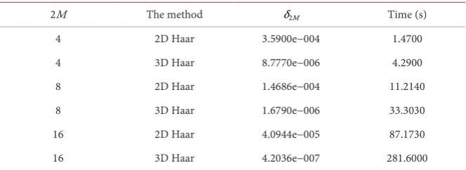
The results for 2D and 3D Haar wavelets method are compared in Table 1 for different values 2M.

We observe from Table 1 that when 2M is not sufficiently large value, means that ∆t_{is not sufficiently small value then the error is big, we can obtain more}

precision by the 3D Haar wavelets than 2D Haar wavelets and in less time. We observe that the precision obtained by 3D Haar wavelets in the case 2M = 4 cannot be obtained for 2D Haar wavelets even one takes 2M = 16 and spends 100 times.

4.2. Poisson Equation

Consider 3D Poisson equation [21]

(

)

2 2 2

2 2 2 , , , 0 , , 1,

u u _{u f x y z} _{x y z}

x y z

∂ ₊∂ ₊∂ ₌ _≤ _≤

∂ ∂ ∂ (39)

(

, ,

)

0

u x y z = _{along the boundaries. Here we have}λ=2,β =2_and

α

=2

and suppose that M1=M2=M3=M.

Now the solution by 3D Haar wavelet is begin using the Equation (12) to ap-proximate problem (16) and considering the initial and boundary conditions at x = 0, y = 0 and z = 0, we get

(

)

( )

( ) ( )

(

)

(

)

(

)

(

)

(

)

(

)

(

)

2 2 2

, , 2, 2, 2,

1 1 1 ₀

2

0 0 0

2 2 3

0 0 0

, , , ,

, , , , , ,

,

M M M

j l i i j l

j l i _y

x x y z

x z y z x y z

u x y z

u x y z a P z P x P y y

y

u x y z u x y z u x y z

x xy z

x x y z

u x y z u x y z u x y z

xz yz xyz

x z y z x y z

= = = ₌

= = = =

= = = = = = =

∂

= +

∂

∂ ∂ ∂

+ − +

∂ ∂ ∂ ∂

∂ ∂ ∂

− − +

∂ ∂ ∂ ∂ ∂ ∂ ∂

∑∑∑

(40) We use the same technique as in (1) to find the unknown terms in Equation (40).

This done in three steps:

(12)

Table 1. Compared the solution of the 2D Heat equation when ∆ =t 1 2M

(

4 1 4

) (

)

t= M− M .

2M The method δ2M Time (s)

4 2D Haar 3.5900e−004 1.4700

4 3D Haar 8.7770e−006 4.2900

8 2D Haar 1.4686e−004 11.2140

8 3D Haar 1.6790e−006 33.3030

16 2D Haar 4.0944e−005 87.1730

16 3D Haar 4.2036e−007 281.6000

2) Substitute the boundary condition when y = 1 in equation resulting 1 and replace this result back into 1.

3) Substitute the boundary condition when z = 1 in equation resulting 2 and replace this result back into 2.

Next the boundary conditions are satisfied

(

)

2 2 2 , ,

{

2,

( )

2

( )

2,

( )

2

( )

2,

( )

2

( )

}

1 1 1

, , M M M j l i i J l ,

j l i

u x y z a P z zq i P x xq j P y yq l

= = =

     

=

∑∑∑

_ − _{ } − _{ } − _

(41) Derivative the Equation (41) we obtain that:

( )

( ) ( )

( )

{

}

2 2 2 2

, , 2, 2 2, 2

2

1 1 1 ,

M M M

j l i i j l

j l i

u _a _{P z} _{zq i h x P y} _{yq l}

x = = =

∂ ₌ _ ₋ _ _ ₋ _

   

∂

∑∑∑

( )

( ) ( )

{

}

2 2 2 2

, , 2, 2 2, 2

2

1 1 1 ,

M M M

j l i i J l

j l i

u _a _{P z} _{zq i} _P _x _{xq j h y}

y = = =

∂ ₌ _ ₋ _{ } ₋ _

   

∂

∑∑∑

( )

{

}

2 2 2 2

, , 2, 2 2, 2

2

1 1 1 ,

M M M

j l i i J l

j l i

u _a _{h z P} _x _{xq j} _{P y} _{yq l}

z = = =

∂ ₌ _ ₋ _{ } ₋ _

   

∂

∑∑∑

We substituting above equations in (39) for any collocation points x yr, k and s

z with

s

∈

{

1 ,

2 ,



,

2 M

}

,

r

∈

{

1 ,

2 ,



,

2 M

}

,

k

∈

{

1 ,

2 ,



,

2 M

}

, we get

(

)

2 2 2

, , , , , , ,

1 1 1 , , for 1 2 ,1 2 ,1 2 , M M M

j l i j l i r k s

j= l= i= a R g s r k s M r M k M

= ≤ ≤ ≤ ≤ ≤ ≤

∑∑∑

(42)

where

( )

( ) ( ) ( )

( )

( ) ( )

( )

(

)

(

)

, , , , , 2 2 2 2

2 2 2 2

, , ,

, , , ,

and

, , , , ,

j l i r k s s k

s r

r k

r k s

R P i s z q i H j r P l k y q l

P i s z q i P j r x q j H l k

H i s P j r x q j P l k y q l

g s r k f x y z

 =_ − _ _ − _

  +_ −  _{ } − _

 + _ −  _{ } − _{ }_    =



(43)

[image:12.595.207.539.106.227.2]

(13)

For the solution by 2D Haar wavelet method we need to divide one of the inter-vals x∈

[

A B1, 1

]

, y∈

[

A B2, 2

]

, z∈

[

A B3, 3

]

into N equal parts and we will

di-vide the interval z∈

[

A B3, 3

]

into N equal parts of length ∆ =z

(

B3−A N3

)

and denote to zs=

(

s− ∆1

)

z s=1,2, , N.

By using Equation (15) and considering the initial-boundary conditions when x = 0, y = 0 and z = 0, we get

(

) (

)

( ) ( ) (

)

(

)

(

)

(

)

(

)

(

)

(

)

(

)

(

)

2 2 2

, 2, 2,

1 1 0 0 0 0 2 2 0 0 2 0 , , , , 2 , , , , , , , , , , , , , , , , M M s

j l j l s

j l s y y s x x s s

x y x y

s x

z z

u x y z a P x P y u x y z

u x y z u x y z

y

y y

u x y z u x y z

x

x x

u x y z u x y z

u x y z

xy z

x y x y z

u x y z

xz yz x z = = = = = = = = = = = − = + _∂ _∂    + −  ∂ ∂    ∂ ∂  + _ − _ ∂ ∂   _∂ _∂  _∂   − − +  ∂ ∂ ∂ ∂  ∂   ∂ − − ∂ ∂

∑∑

(

)

(

)

2 3 0 0 , , , , , s s

y x y

u x y z u x y z

xyz

y z ₌ x y z _{= =}

∂ ∂

+

∂ ∂ ∂ ∂ ∂

(44) where the element aj l, is constant in the subinterval z∈

(

z zs, s+1

]

.

Next the boundary conditions when x = 1, y = 1 and z = 1 are satisfied

(

)

(

₍

_{) (}

)

) (

)(

)

( )

{

}

2

2 2

, 2, 2 2, 2

1 1

1

, , 1 , ,

1 2 2

,

s s s s

s s

M M

j l J l

j l

z z z z z z z

u x y z u x y z

z

a P x xq j P y yq l

= =    −  − − −   = −  + − −             ×

∑∑

_ − _{ } − _ (45)

from Equation (45), we get

(

)

(

)

(

) (

)(

)

( )

{

}

2 2 2 2 2 2 2

, 2, 2

1 1

1 2 2

,

s

s s s s

s z z

M M

j l j l j l

z z z z z z z

u u

z

x x

a h x P y yq l

= = =    −  − − − ∂ _{= −} ∂ ₊_ ₋ _  ₋  ∂  ∂ _ _   ×

∑∑

_ − _

(

)

(

)

(

) (

)(

)

( )

( ) ( )

{

}

2 2 2 2 2 2 2

, 2, 2

1 1

1 2 2

,

s

s s s s

s z z

M M

j l J l

j l

z z z z z z z

u u

z

y y

a P x xq j h y

= = =    −  − − − ∂ ∂   = −  + − − ∂  ∂ _ _   ×

∑∑

_ − _

( )

{

}

2 2 2

, 2, 2 2, 2

2

1 1 ,

M M

j l J l

j l

u _a _P _x _{xq j} _{P y} _{yq l}

z = =

∂ ₌ _ ₋ _{ } ₋ _

   

∂

∑∑

We substituting above equation in (39) for any collocation points x yr, k with

{

1,2, ,2

}

(14)

(

)

2 2

, , , ,

1 1 , , for 1 2 ,1 2 ,1 , M M

j l j l r k

j= l= a R g r k s r M k M s N

= ≤ ≤ ≤ ≤ ≤ ≤

∑∑

(46)

where

( )

(

)

_{( ) ( )}

_{( )}

( )

(

)

_{( )}

_{( ) ( )}

(

)

(

)

₍

₎

(

)

, , , 2 2 2 2

2

2 2

2

2 2

2

, ,

2

, ,

1

, ,

2 2

1

, , ,

2 2

and

, , , , 1

1

1 1

s r k

j l r k r k

s

k

s

r

r k s

s z z x x y y

s z

R P j r x q j P l k y q l

z z

z

H j r P l k y q l

z z

z _{P j r} _{x q j H l k}

z u

g r k s f x y z

z x

z u

z y

= = = =_ −  _{ } − _

 _∆ _∆ ₋ 

+ −  _ − _

 

 

 _∆ _∆ ₋ 

+ − _{ } − _

 

 

 ∆ ∂

= − − 

− ∂

 

 

 _∆ _∂

− −_ _

− ∂

 

  , ,

,

s r k

z x x y y

= = =

                  

(47)

The solution u (x, y, z) get it from the Equation (45).

4.2.3. Numerical Results

Solve (39) for f x y z

(

, ,

)

=sin

( ) ( ) ( )

πx sin πy sin πz is:

(

, ,

)

₃_π12sin

( ) ( ) ( )

π sin π sin π ,

u x y z = − x y z

Also we use the MATLAB norm error δ2M =norm u u

(

− ex,2 2

)

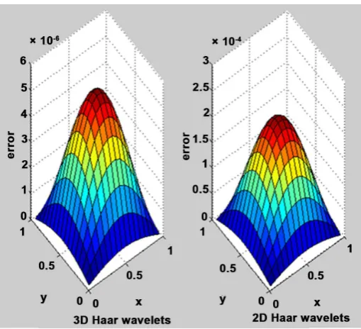
M . we

plot-ted in Figure 1 the error δ2M for 2M = 16 near from the last time z = 1 to illu-strate the impact of error accumulation on the solution by 2D Haar wavelets.

[image:14.595.226.538.100.303.2]

Results obtained using 2D and 3D Haar wavelets method are compared in

Table 2 for different values 2M.

In 2D Haar wavelets method, We can reduce the error and increase accuracy by increasing the subdivisions for the time (t) or the interval z∈

[

A B3, 3

]

in

examples (1) and (2) and minimize the value of ∆t or ∆z With the installa-tion’s divisions for x∈

[

A B1, 1

]

and y∈

[

A B2, 2

]

according to formula of Haar

wavelets, This helps increase the accuracy of the solution in the 2D Haar wave-lets method, But it requires more time to get on the solution as shown in Table 3.

All computation was made by using MATLAB Language, Intel®, core™ I3-2330M CPU, 2.00 GB (Memory), 2.20 GHz (Processor).

5. Conclusions

(15)

[image:15.595.246.501.68.300.2]

Figure. 1. The error δ16 at z=31 32 by using 3D and 2D Haar wavelets method.

Table 2. Compared the solution of the 3D Poisson equation when ∆ =z 1 2M and

(

4 1 4

) (

)

z= M− M .

2M The method δ2M Time (s)

4 2D Haar 3.1669e−004 1.4000

4 3D Haar 7.7797e−005 3.2800

8 2D Haar 1.8481e−004 10.6220

8 3D Haar 1.0420e−005 25.5220

16 2D Haar 5.3391e−005 84.2600

16 3D Haar 1.3243e−006 251.632

Table 3. Illustrates the convergence of the solution of the 3D Poisson equation by using the 2D Haar wavelets method with 2M =8_{and for different values} ∆z_.

z

∆ δ2M Time (s)

( )

1 2M 1.8481e−004 10.6220

( )

1 4M 5.2623e−005 21.6400

( )

1 8M 1.2907e−005 42.7320

(2M) as note in Table 1 and Table 2. Also when 2M = 32, 2M = 64 …, we can obtain the results closer to the exact values.

[image:15.595.208.540.383.503.2] [image:15.595.206.540.548.617.2]

(16)

DOI: 10.4236/oalib.1104496 16 Open Access Library Journal The main benefits of the proposed method are its simplicity (already a small number of grid pointsguarantee the necessary accuracy) and universality (the same approach is applicable for a wide class of PDEs). The method is very con-venient for solving boundary value problems, since the boundary conditions are taken into account automatically. For numerical calculations useful are the ma-trix programs of MATLAB. The most time-consuming procedure is to calculate the integrals (4). In this paper only linear problems were considered, but the method is applicable also for nonlinear PDEs.

Acknowledgements

This work was carried out when third author was visiting the mathematics de-partment at Nantes University, France, with the support of ministry of higher education and scientific research, Iraq. The authors Ekhlass S. and Qasim F. would like to express their gratitude to Professor Abdeljalil Nachaoui for intro-ducing to the subject and for giving all necessary support to complete this work and for his hospitality.

References

[1] Zhi, S., Deng, L.-Y. and Qing, J.C. (2007) Numerical Solution of Differential Equa-tions by Using Haar Wavelets. Proceeding of the International Conference on Wavelet Analysis and pattern Recognition, 2-4 NovEMBER 2007, Beijing, China, 1039-1044. https://doi.org/10.1109/ICWAPR.2007.4421585

[2] Bertoluzza, S. (1977) An Adaptive Collocation Method Based on Interpolating Wavelets. In: Dahmen, W., Kurdila, A.J. and Oswald, P., Eds., Multi-Scale Wavelet Methods for Partial Differential Equations, Academic Press, San Diego, 109-135. [3] Beylkin, G. and Keiser, J.M. (1977) An Adaptive Pseudo-Wavelet Approach for

Solving Nonlinear Partial Differential Equations. In: Dahmen, W., Kurdila, A.J. and Oswald, P., Eds., Multi-Scale Wavelet Methods for Partial Differential Equations, Academic Press, San Diego, 137-197.

[4] Chen, X., Xiang, J., Li, B. and He, Z. (2010) A Study of Multiscale Wavelet-Based Elements for Adaptive Finite Element Analysis. Advances in Engineering Software, 41, 196-205. https://doi.org/10.1016/j.advengsoft.2009.09.008

[5] Hariharan, G., Kannan, K. and Sharma, K.R. (2009) Haar Wavelet Method for Solving Fisher’s Equation. Applied Mathematics and Computation, 211, 284-292. https://doi.org/10.1016/j.amc.2008.12.089

[6] Arora, S., Singh, I., Brar, Y.S. and Kumar, S. (2015) Comparative Study of Haar Wavelet with Numerical Methods for Partial Differential Equations. International Journal of Pure and Applied Mathematics, 101, 489-503.

[7] Arbabi, S., Nazari, A. and Darvishi, M.T. (2017) A Two-Dimensional Haar Wavelets Method for Solving Systems of PDEs. Applied Mathematics and Computation, 292, 33-46. https://doi.org/10.1016/j.amc.2016.07.032

[8] Wang, X.J., Nan, B., Zhu, J. and Koeppe, R. (2014) Regularized 3d Functional Re-gression for Brainimage Data via Haar Wavelets. The Annals of Applied Statistics, 8, 1045-1064. https://doi.org/10.1214/14-AOAS736

(17)

DOI: 10.4236/oalib.1104496 17 Open Access Library Journal of Bucharest. Series A Applied Mathematics and Physics, 78, 111-126.

[10] Chun, Z. and Zheng, Z. (2007) Three-Dimensional Analysis of Functionally Graded Plate Based on the Haar Wavelet Method. Acta Mechanica Solida Sinica, 20, 95-102. https://doi.org/10.1007/s10338-007-0711-3

[11] Majak, J., Pohlak, M., Eerme, M. and Lepikult, T. (2009) Weak Formulation Based Haar Wavelet Method for Solving Differential Equations. Applied Mathematics and Computation, 211, 488-494. https://doi.org/10.1016/j.amc.2009.01.089

[12] Castro, L.M.S., Ferreira, A.J.M., Bertoluzza, S., Patra, R.C. and Reddy, J.N. (2010) A Wavelet Collocation Method for the Static Analysis of Sandwich Plates Using a Layerwise Theory. Composite Structures, 92, 1786-1792.

https://doi.org/10.1016/j.compstruct.2010.01.021

[13] Chen, C. and Hsiao, C.H. (1997) Haar Wavelet Method for Solving Lumped and Distributed Parameter Systems. IEE Proceedings-Control Theory and Applications, 144, 87-94. https://doi.org/10.1049/ip-cta:19970702

[14] Lepik, Ü. (2008) Solving Integral and Differential Equations by the Aid of Nonuni-form Haar Wavelets. Applied Mathematics and Computation, 198, 326-332. https://doi.org/10.1016/j.amc.2007.08.036

[15] Lepik, Ü. (2008) Haar Wavelet Method for Solving Higher Order Differential Equa-tions. International Journal of Mathematics and Computation, 1, 84-94.

[16] Lepik, Ü. (2005) Numerical Solutions of Differential Equations Using Haar Wave-lets. Mathematics and Computers in Simulation, 68, 127-143.

https://doi.org/10.1016/j.matcom.2004.10.005

[17] Lepik, Ü. (2007) Numerical Solution of Evolution Equations by the Haar Wavelet Method. Applied Mathematics and Computation, 185, 695-704.

https://doi.org/10.1016/j.amc.2006.07.077

[18] Lepik, Ü. (2011) Solving PDFs with the Aid of Two-Dimensional Haar Wavelets. Computers and Mathematics with Applications, 61, 1873-1879.

https://doi.org/10.1016/j.camwa.2011.02.016

[19] AL-Rawi, E.S. and Qasim, A.F. (2014) CAS Wavelets for Solving General Two Di-mensional Partial Differential Equations of Higher Order with Application. Inter-national Journal of Enhanced Research in Science Technology & Engineering, 3, 496-507.

[20] Shiralashetti, S.C., Angadi, L.M., Deshi, A.B. and Kantli, M.H. (2016) Haar Wavelet Method for the Numerical Solution of Benjamin-Bona-Mahony Equations. Journal of Information and Computing Science, 11, 136-145.