Different Forms Biasing Parameter for Generalized
Ridge Regression Estimator
Taiwo Stephen Fayose
Department of Mathematics and Statistics Federal Polytechnic
Ado- Ekiti, Nigeria
Kayode Ayinde
Department of Statistics Federal University of Technology
Akure, Nigeria
ABSTRACT
The concept of different forms on the basis of original, minimum, maximum and measures of locations of eigen values of XIX of the design matrix in regression analysis was
introduced into estimating the biasing or ridge parameter of the generalized ridge estimator of linear regression model with multicollinearity problem. This resulted into some proposed biasing parameters having considered existing seven (7) biasing parameters of the Generalized Ridge Regression (GRR) estimator. Their performances were examined and compared with the Ordinary Least Square (OLS) estimator and the existing (parent / original) biasing parameters of GGR estimator so as to identify the one(s) that would produce efficient estimates of the model parameters. Monte Carlo experiments were conducted 5000 times on two linear regression models with three and six explanatory (p = 3 and p = 6) variables under six (6) levels of multicollinearity ( = 0.8, 0.9, 0.95, 0.99, 0.999, 0.9999), three (3) levels of standard error (σ = 1, 5 and 10) and seven (7) levels of sample sizes (n = 10, 20, 30, 50, 100, 150,
250).
The estimators were compared using Mean Square Error (MSE) criterion.Results showed that the proposed different forms biasing parameters frequently perform more efficiently than the parent form; and that the different form of minimum of eigen values of XIX using the generalized ridge parameter of Batach et al. (2008) often produces efficient estimates of linear regression parameter with multicollinearity problem.
General Terms
Linear Regression Model, Multicollinearity,
Keywords
Different Forms Biasing parameter, Ordinary Least Square Estimator, Generalized Ridge Regression Estimator, Mean Square Error
1.
INTRODUCTION
Multiple linear regression models assess relationship between a dependent variable and a set of independent (explanatory) variables. To estimate the parameters of regression model, the Ordinary Least Squares (OLS) Estimator has been most popularly used and discussed (Bowerman and O’ Connell, 1990). The estimator has some very attractive statistical properties when none of the assumptions of the classical linear regression model is violated; the OLS is BLUE (Best Linear Unbiased Estimator). This has made the OLS estimator to be the most powerful and popular estimator of regression model. One of the common violations of the assumptions is that of the dependence of the explanatory variables often refers to as multicollinearity. OLS estimator in the presence of multicollinearity is BLUE (Gujarati, 2003).
The consequences of multicollinearity are often very serious.
These include the inability of the OLS estimators to provide the unique effects of individual variables in the regression model and their large sampling variances. These often lead to erroneous conclusion in hypothesis testing and predictions (Johnston, 1987; Gujarati, 1995). Furthermore, the OLS estimators yield regression coefficients whose absolute values are too large and whose signs may actually reverse with negligible changes in the data (Buonaccorsi, 1996). The problem of multicollinearity in regression analysis can have effects on the estimated least square regression coefficients, computational accuracy, estimated standard deviation of the least squares regression coefficients, t-test, extra sum of squares, fitted values and predictions and coefficients of determination (Maddala, 2005).
Maddala (2005) opined that once multicollinearity is detected in the data, a natural question is “how to estimate the coefficients in its presence?” Several methods of estimating regression parameters in the presence of multicollinearity include ridge regression, partial least square regression and principal component regression (Abdi, 2013). The most widely recognized and immensely used technique is the Ridge Regression (Vinod and Ullah, 1981) proposed by Hoerl and Kennard (1970a). The authors showed that a ridge estimator has smaller Mean Square Error (MSE) than that of the OLS estimator making the estimator to be more efficient. The ridge estimator is a modification of the least square method that allows biased estimator of the regression coefficients. These biased estimators are preferred over unbiased ones since they have smaller mean square errors.
However to achieve this, the biasing or ridge parameter, k, plays a very significant role to control the bias of the regression toward the mean of the dependent variable. A major problem of ridge regression parameter is the choice of k. Therefore, Hoerl and Kennard (1970a) proposed the Generalized Ridge Regression (GRR) estimator that accommodates separate ridge parameters for each explanatory variable. Several ridge parameters, ks, have been proposed by
different authors. These include Nomura (1988), Troskie and Chalton (1996), Firinguetti (1999), Batach et. al (2008), Dorugade (2016) and Lukman and Ayinde (2017).
Consider the standard regression model:
U
X
Y
(1)Where
X
is an n x p matrix with full rank,Y
is a n x 1 vector of dependent variable,
is a p x 1 vector of unknown parameters, andU
is the error term that0
)
(
U
E
andE
(
U
U
)
2In.Y
X
X
X
I I OLS1
)
(
ˆ
(2)The Generalized Ridge Regression Estimator (GRRE) is defined as:
Y
X
KI
X
X
I IRidge
1
)
(
ˆ
(3)Where
X X
1 is a p x p product matrix of explanatory variables,X Y
1 is a p x 1 vector of the product of dependent and explanatory variables, K = diagonal (k
1,k
2,…,k
p),. ki≥ 0. i = 1, 2---, p. K is a non-negative constant. It is called biasing or ridge parameter. It is observed that when k = 0, (3) returns to OLS estimator (John, 1998).
Suppose the response variable y is centered and the regressors X’s are standardized. Let and T be the matrices of eigen values and eigen vectors of
respectively such that
= = diagonal (
λ1, λ2, …λp), where λ1 representsthe ith eigenvalue of
and = =I
p. The equivalentmodel for equation (1) becomes:
y = Zα + u (4) (4) where Z = XT such that
= and
α =T′β.Consequently, the OLS estimator of α becomes:
OLS = (
)-1
= -1
(5) (5)
The relationship between the OLS estimator of β and α is given as:
OLS= T OLS. (6) (6)
The MSE of the ridge estimator is:
MSE(
ˆ
ridge)
=
p i pi i i i i i i i
k
k
k
1 1 2
2 2 2 2
)
ˆ
(
ˆ
ˆ
)
ˆ
(
ˆ
(7)while the MSE of the OLS estimator is:
MSE
p i i OLS 1 21
ˆ
)
ˆ
(
(8)where
1,
2,
,
pare the eigen values ofX
X
1
.
k
ˆ
is the estimator of the ridge parameter k,
ˆ
iis the ith element of the vector
ˆ
defined in (5).2.
LITERATURE REVIEW
2.1 Biasing or Ridge Parameter
Ridge regression focalizes on the use of the biased parameter K which produces estimation with a smaller Mean Square Error. Hoerl and Kennard (1970a,b) suggested the optimum ridge parameter whose estimator is defined as:
2 2
ˆ
ˆ
)
(
ˆ
i iHK
k
KGRHK
, i = 1, 2, 3, p. (9)where
ˆ
2 =p
n
e
n i i
1 2and it is the Mean Square Error from
the OLS regression,
i is the ith element of the vector
ˆ
from OLS regression defined in (5), p is the number of regressors and n is the sample size.Nomura (1988) proposed another ridge parameter whose estimator is defined as:
2 1 2 2 2 2ˆ
ˆ
1
1
ˆ
ˆ
)
(
ˆ
i i i iN
k
KGRN
(10)where
iis the ith eigen value ofX X
1 .Troskie and Chalton (1996) proposed another ridge parameter whose estimator is defined as:
)
ˆ
ˆ
(
ˆ
)
(
ˆ
2 2 2
i i i iTC
k
KGRTC
(11)Firinguetti (1999) also proposed another ridge parameter whose estimator is defined as:
2 2 2
ˆ
)
(
ˆ
(
ˆ
)
(
ˆ
p
n
F
k
KGRF
i i i i
(12)where p is the number of regressors and n is the sample size. Batach et. al (2008) proposed another ridge parameter whose estimator is defined as:
2 2 2 1 2 4 2 2 4 2 2ˆ
2
ˆ
ˆ
ˆ
6
ˆ
4
ˆ
ˆ
)
(
ˆ
i i i i i ii i
BAO
k
KGRB
(13)
Dorugade (2016) proposed another ridge parameter whose estimator is defined as:
2 2
ˆ
ˆ
2
)
(
ˆ
i i iD
k
KGRD
(14)Lukman and Ayinde (2017) proposed another ridge parameter in line with Lawless and Wang (1976) and its estimator is defined as: 2 2
ˆ
ˆ
)
(
ˆ
i i iLA
k
KGRLA
(15)Thus, the seven (7) parent (original) biasing parameters for the Generalized Ridge Regression estimator were considered in this research study.
2.2 Different forms Biasing or Generalized
Ridge Parameters
seven (7) biasing parameters for GRR are proposed. Their estimators are defined as follows:
2 1 2 2 2 2ˆ
ˆ
1
1
ˆ
ˆ
)
(
ˆ
i Min i Min ik
KGRNMI
(16)where
Min= Min(
i), i=1, 2, 3,…,p
2 1 2 2 2 2ˆ
ˆ
1
1
ˆ
ˆ
)
(
ˆ
i Max i Max ik
KGRNMA
(17)where
Max= Max(
i), i=1, 2, 3,…,p
2 1 2 2 2 2ˆ
ˆ
1
1
ˆ
ˆ
)
(
ˆ
i MR i MR ik
KGRNMR
(18)where
MR =2
Max Min
MR
2 1 2 2 2 2ˆ
ˆ
1
1
ˆ
ˆ
)
(
ˆ
i AM i AM ik
KGRNAM
(19) where 11
p AM i ip
2 1 2 2 2 2ˆ
ˆ
1
1
ˆ
ˆ
)
(
ˆ
i Median i Median ik
KGRNMD
(20)where
Median= Median(
i), i=1, 2, 3,…,p
2 1 2 2 2 2ˆ
ˆ
1
1
ˆ
ˆ
)
(
ˆ
i GM i GM ik
KGRNGM
(21)where
1
1 2
...
1 2...
2p p GM p
2 1 2 2 2 2ˆ
ˆ
1
1
ˆ
ˆ
)
(
ˆ
i HM i HM ik
KGENHM
(22) where 11
HM p i ip
In the same way, using the parent ridge parameter, k, by Troskie and Chalton (1996)in equation (11); the parent ridge parameter, k, by Firinguetti (1999) in equation (12); the parent ridge parameter, k, by Batach et. al (2008)in equation (13); the parent ridge parameter, k, by Dorugade (2016) in equation (14); and the parent ridge parameter, k, by Lukman and Ayinde (2017)in equation (15), other different forms of biasing parameters were also proposed.
3.
SIMULATION STUDY
3.1 Model and Data Generation
Consider a multiple linear regression model of the form:
(23)
t = 1,2,…,n ; p = 3, 6.
where
.
, t=1,2,…,n; i =1,2,...,p are fixed regressors.The error terms were generated to be normally distributed with mean zero and variance
. In this
study, 2 values were 1, 25 and 100. The model was studied with fixed regressors, Xit, i = 1, 2, ..., p; t = 1, 2, ..., n such thatthere exist different levels of multicollinearity among the regressors. Following McDonald and Galarneau (1975), Wichern and Churchill (1978), Gibbons (1981), Kibria (2003), Dorugade and Kashid (2010), Dorugade (2016), and Lukeman and Ayinde (2017); the equation to generate the explanatory variables in given as:
(24) t=1, 2, 3,…, n. i=1, 2,…p.
where is independent standard normal distribution with mean zero and unit variance, is the correlation between any two explanatory variables and p is the number of explanatory variables. The values of were taken as 0.8, 0.9, 0.95, 0.99, 0.999 and 0.9999 respectively. In this study, the number of explanatory variables (p) were three (3) and six (6).
100, 150 and 250. At a specified value of n, p and σ, the fixed Xs are first generated; followed by the U, and the values of Y
are then obtained using the regression model. This Us were
generated 5000 times and the Ys were determined. The Ys and
the Xs were then treated as real life dataset while the
estimators were applied.
3.2 Criterion for Comparison and oChoice
of most efficient stimator(s)
The performances of both the existing and the proposed biasing parameters of GRR estimators were done by computing the Mean Square Error (MSE) of the model parameters. This has been commonly used by Hoerl and Kennard (1970b), Hoerl et al. (1975), Lawless and Wang (1976), Saleh and Kibria (1993), Kibria (2003), Khalaf and Shukur (2005), Alkhamisi and Shukur (2008), Mansson et al. (2010), Kibria and Banik (2016), Dorugade (2016) and Lukman and Ayinde (2017) for this kind of study. The Mean Square Error for each estimator over the 5000 replications was computed as:
pi j
i ij
MSE
1 5000
1
2
ˆ
5000
1
)
ˆ
(
(25)where
ˆ
ij is ith element of the estimator in the jth replication which gives the estimate of
i for the estimatorbeing considered.
i are the true value of the parameter previously mentioned.A statistical package, Time Series Processor (TSP, 5.0), was used to write the program to compute the Mean Square Error (MSE) of all these estimators. At a particular level of error variance, multicollinearity, and sample size, the MSE of each estimator was ranked using computer Statistical Package for the Social Sciences (SPSS 17.0) on the basis of their MSE values for each parent ridge biasing parameter and later for the overall with the OLS estimator and GRR with ridge parameter of Hoerl and Kennard (1970b). The number of times each form of biasing parameter has minimum MSE (rank 1) was counted over the levels of multicollinearity and error variance at each parent biasing parameter and later overall. The most frequent efficient estimator is expectedly to have the highest number of counts, the mode.
4.
RESULTS AND DISCUSSION
The results from original biasing parameter and that of their different forms are presented for each parent ridge parameter and also the overall having counted the number of times the MSE is minimum over the levels of multicollinearity and standard error are presented as follows:
4.1 Results with Nomura (1988) GRR
Estimator
[image:4.595.310.549.72.326.2] [image:4.595.317.536.645.732.2]The number of times the different forms of Nomura (1988) produced minimum MSE when p = 3 and p = 6 is presented in Table 1.
Table 1: Number of times the different forms of Nomura (1988) produced minimum MSE
p Estimators
Sample Sizes
10 20 30 50 100 150 250 Total
KGRN 0 0 0 0 0 0 0 0
3
KGRNMI 3 7 7 9 10 10 12 58
KGRNMA 0 0 0 0 0 0 0 0
KGRNMR 0 0 0 0 0 0 0 0
KGRNAM 2 0 0 0 0 0 0 2
KGRNMD 7 6 6 5 3 2 2 31
KGRNGM 4 3 3 3 3 4 3 23
KGRNHM 2 2 2 1 2 2 1 12
6
KGRN 0 0 0 0 0 0 0 0
KGRNMI 1 4 4 7 9 10 10 45
KGRNMA 0 0 0 0 0 0 0 0
KGRNMR 2 0 0 0 0 0 0 2
KGRNAM 12 8 8 6 6 5 3 48
KGRNMD 2 2 2 0 1 2 1 10
KGRNGM 0 4 2 3 2 1 3 15
KGRNHM 1 0 2 2 0 0 1 6
Note: The most frequent efficient estimator is bolded over the levels of sample size.
From Table 1, it can be observed the GRR estimator of Nomura (1988) with minimum eigen values of
X
1X
produced the highest number of times MSE is minimum when p = 3. This is followed by the median and the geometric mean versions of eigen values ofX
1X
of Nomura (1988). Thus when p=3, the GRR estimator of Nomura (1988) with minimum of eigen value is the most frequent efficient estimator except when the sample size is very small, n=10. At this instance, the most frequent efficient GRR estimator of Nomura (1988) is the one that uses the median of eigen values ofX
1X
. The performances of that of Harmonic mean is fair in all the sample sizes. Figure 1 illustrates these. When p = 6, the GRR estimator of Nomura (1988) with arithmeticmean eigen values ofX
1X
produced the highest number of times MSE is minimum. This is followed by the minimum and the geometricmean versions of eigen values ofX
1X
of Nomura (1988). Thus, the GRR estimator of Nomura (1988) with minimum of eigen value is still the most frequent efficient estimator except when the sample size is small, n<=30. At thse instances, the most frequent efficient GRR estimator of Nomura (1988) is the one that uses the arithmetic mean of eigen values ofX
1X
. Moreover, the performances of that of geometric and median are fair over the levels of the sample sizes. All these are illustrated in Figure 1.Figure 1: Number of Counts at which MSE is Minimum for the different forms of GRR estimator of Nomura
(1988)
0 20 40 60 80 KGRN/KGRNMR/KGRN…
KGRNGM KGRN/KGRNMA KGRNMD KGRNAM
p
=3
p
=6
Number Of Counts
Esti
m
ato
4.2 Results with Troskie and Chalton
(1996)GRR Estimator
[image:5.595.317.556.95.227.2]Table 2 presents the number of times the different forms of Troskie and Chalton (1996) produced minimum MSE when counted over the levels of multicollinearity and standard error levels when p = 3 and p = 6. From Table 2, it can be observed the GRR estimator of Troskie and Chalton (1996) with maximum eigen values of
X
1X
produced the highest number of times MSE is minimum when p = 3. This is followed by the minimum and the original versions of eigen values ofX
1X
of Troskie and Chalton (1996). Furthermore when p = 6, the GRR estimator of Troskie and Chalton (1996) with originl eigen values ofX
1X
produced the highest number of times MSE is minimum. This is followed by the harmonic mean, the minimum and maximum versions of eigen values ofX
1X
of Troskie and Chalton (1996).Table 2: Number of times the different forms of Troskie andChalton (1996) produced minimum MSE
p Estimato rs
Sample Sizes 1
0 2 0
3 0
5 0
10 0
15 0
25 0
Tot al
3
KGRTC 0 0 0 1 1 0 4 6
KGRTC MI
2 5 5 6 7 10 8 43
KGRTC MA
1 5
1 1
1 1
1 0
8 6 6 67
KGRTC MR
0 1 0 0 1 0 0 2
KGRTCA M
0 0 0 0 0 0 0 0
KGRTC MD
0 0 1 0 1 0 0 2
KGRTCG M
1 0 0 0 0 2 0 3
KGRTCH M
0 1 1 1 0 0 0 3
6
KGRTC 1
8 1 8
1 4
1 8
16 17 17 118
KGRTC MI
0 0 0 0 1 1 0 2
KGRTC MA
0 0 2 0 0 0 0 2
KGRTC MR
0 0 0 0 0 0 0 0
KGRTCA M
0 0 1 0 0 0 0 1
KGRTC MD
0 0 0 0 0 0 0 0
KGRTCG M
0 0 0 0 0 0 0 0
KGRTCH M
0 0 1 0 1 0 1 3
Note: The most frequent efficient estimator is bolded over the levels of sample size.
Thus when p=3, the GRR estimator of Troskie and Chalton (1996) with maximun of eigen value is the most frequent efficient estimator except when the sample size is large, n>100. At these instances, the most frequent efficient GRR estimator of Troskie and Chalton (1996) is the one that uses the minimum of eigen values of
X
1X
. Moreover when p=6, the original biasing parameter of Troskie and Chalton [image:5.595.54.284.294.662.2](1996) estimator is the most frequent efficient estimator. All these are illustrated in Figure 2.
Figure 2: Number of Counts at which MSE is Minimum for the different forms of GRR estimator of Troskie and
Chalton (1996).
4.3 Results with Firinguetti (1999)
GRREstimator
The number of times the different forms of Firinguetti (1999) produced minimum MSE when counted over the levels of multicollinearity and standard error levels when p = 3 and p = 6 is presented in Table 3.
p Estimato rs
Sample Sizes 1
0 2 0
3 0
5 0
10 0
15 0
25 0
Tot al
3
KGRF 0 0 0 0 0 0 1 1
KGRFMI 0 3 3 3 3 3 2 17
KGRFM A
1 5
1 3
1 3
1 3
10 10 10 84
KGRFM R
0 1 0 0 3 0 1 5
KGRFA M
0 0 1 1 0 3 2 7
KGRFM D
0 0 0 0 1 0 0 1
KGRFG M
1 0 0 0 0 1 1 3
KGRFH M
2 1 1 1 1 1 1 8
6
KGRF 3 0 0 1 2 2 2 10
KGRFMI 0 1 0 0 0 0 0 1
KGRFM A
1 5
1 3
1 6
1 3
13 13 12 95
KGRFM R
0 1 1 1 0 0 2 5
KGRFA M
0 1 1 2 2 2 1 9
KGRFM D
0 0 0 1 0 1 0 2
KGRFG M
0 1 0 0 1 0 1 3
KGRFH M
0 1 0 0 0 0 0 1
Note: The most frequent efficient estimator is bolded over the levels of sample size.
From Table 3, it can be observed the GRR estimator of Firinguetti (1999) with maximum eigen values of
X
1X
produced the highest number of times MSE is minimum when p = 3 and p=6.Thus, Moreover when p=6, the GRR estimator of Firinguetti
0 50 100 150 KGRTCAM
KGRTCGM/KGRTCHM KGRTCMI KGRTCMD/KGRTCGM KGRTCMI/KGRTCMA KGRTC
p
=3
p
=6
Number Of Counts
Esti
m
ato
[image:5.595.314.544.345.676.2](1999) with maximum eigen value is the most frequent efficient estimator. This is further illustrated in Figure 3.
Figure 3: Number of Counts at which MSE is Minimum for the different forms of GRR estimator of Firinguetti
(1999).
4.4 Results with Batach et al (2008)
GRR Estimator
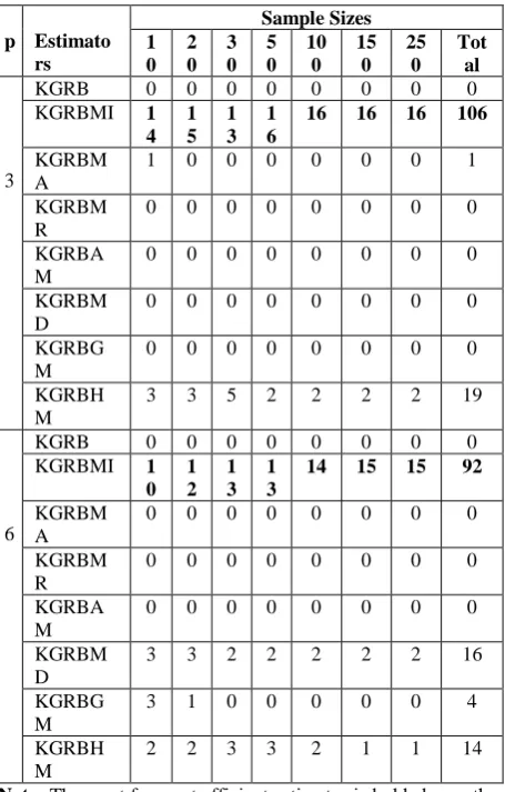
[image:6.595.317.553.137.233.2]The number of times the different forms of Batach et al (2008) produced minimum MSE when counted over the levels of multicollinearity and standard error levels when p = 3 and p = 6 is presented in Table 4.
Table 4: Number of times the different forms of Batach et al (2008) produced minimum MSE
p Estimato rs
Sample Sizes 1
0 2 0
3 0
5 0
10 0
15 0
25 0
Tot al
3
KGRB 0 0 0 0 0 0 0 0
KGRBMI 1
4 1 5
1 3
1 6
16 16 16 106
KGRBM A
1 0 0 0 0 0 0 1
KGRBM R
0 0 0 0 0 0 0 0
KGRBA M
0 0 0 0 0 0 0 0
KGRBM D
0 0 0 0 0 0 0 0
KGRBG M
0 0 0 0 0 0 0 0
KGRBH M
3 3 5 2 2 2 2 19
6
KGRB 0 0 0 0 0 0 0 0
KGRBMI 1
0 1 2
1 3
1 3
14 15 15 92
KGRBM A
0 0 0 0 0 0 0 0
KGRBM R
0 0 0 0 0 0 0 0
KGRBA M
0 0 0 0 0 0 0 0
KGRBM D
3 3 2 2 2 2 2 16
KGRBG M
3 1 0 0 0 0 0 4
KGRBH M
2 2 3 3 2 1 1 14
Note: The most frequent efficient estimator is bolded over the levels of sample size.
From Table 4, it can be observed the GRR estimator of Batach et al (2008) with minimum eigen values of
X
1X
produced the highest number of times MSE is minimum when p = 3 and p=6; and so it the most frequent efficient estimator of Batach et al (2008). This is illustrated pictorially in Figure 4.Figure 4: Number of Counts at which MSE is Minimum for the different forms of GRR estimator of Batach et al
(2008).
4.5 Results with Dorugade (2016) GRR
Estimator
In Table 5, the number of times the different forms of Dorugade (2016) produced minimum MSE when counted over the levels of multicollinearity and standard error levels when p = 3 and p = 6 is presented.
From Table 5, it can be observed the biasing parameter of the GRR estimator of Dorugade (2016) with minimum eigen value of
X
1X
is the most frequent efficient estimator when the sample size is large and that it is either the one with minimum eigen value or the parent ridge parameter when the sample size is small. Figure 5 illustrates these.Note: The most frequent efficient estimator is bolded over the levels of sample size.
Figure 5: Number of Counts at which MSE is Minimum for the different forms of GRR estimator of Dorugade
(2016).
4.6 Results with Lukman and Ayinde
(2017) GRR Estimator
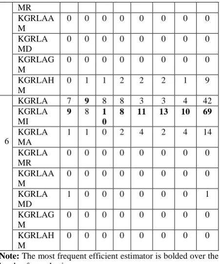
The number of times the different forms of Lukman and Ayinde (2017) produced minimum MSE when counted over the levels of multicollinearity and standard error levels when p = 3 and p = 6 is presented in Table 6.
Table 6: Number of times the different forms of Lukman and Ayinde (2017) produced minimum MSE
p Estimato rs
Sample Sizes 1
0 2 0
3 0
5 0
10 0
15 0
25 0
To tal
3
KGRLA 1
0
6 6 2 2 2 2 26
KGRLA MI
8 7 7 8 8 8 8 54
KGRLA MA
0 4 4 6 6 6 7 33
KGRLA 0 0 0 0 0 0 0 0
0 20 40 60 80 100 KGRF/KGRFMD
KGRFMR KGRFHM KGRFMA KGRFMD KGRFMR KGRF
p
=3
p
=6
Number Of Counts
Esti
m
ato
rs
0 20 40 60 80 100 120 KGRB/KGRBMR/KGRBA…
KGRBHM KGRB/KGRBMA/KGRBM…
KGRBHM KGRBMI
p
=3
p
=6
Number Of Counts
Esti
m
ato
rs
0 20 40 60 80 KGRDMR/KGRDAM/KG…
KGRD KGRDMR/KGRDAM/KG…
KGRD
p
=3
p
=6
Number Of Counts
Esti
m
ato
[image:6.595.55.283.377.734.2] [image:6.595.316.548.434.518.2]MR KGRLAA M
0 0 0 0 0 0 0 0
KGRLA MD
0 0 0 0 0 0 0 0
KGRLAG M
0 0 0 0 0 0 0 0
KGRLAH M
0 1 1 2 2 2 1 9
6
KGRLA 7 9 8 8 3 3 4 42
KGRLA MI
9 8 1 0
8 11 13 10 69
KGRLA MA
1 1 0 2 4 2 4 14
KGRLA MR
0 0 0 0 0 0 0 0
KGRLAA M
0 0 0 0 0 0 0 0
KGRLA MD
1 0 0 0 0 0 0 1
KGRLAG M
0 0 0 0 0 0 0 0
KGRLAH M
0 0 0 0 0 0 0 0
Note: The most frequent efficient estimator is bolded over the levels of sample size
From Table 6, it can be observed the GRR estimator of Lukman and Ayinde (2017) with minimum eigen values of
X
[image:7.595.313.543.69.259.2]X
1 is generally the most frequent efficient estimator. However at small sample sizes, the original biasing parameter occasionally becomes the most frequent efficient estimator. This is further presented pictorially in Figure 6.Table 5: Number of times the different forms of Dorugade (2016) produced minimum MSE
p Estimato rs
Sample Sizes 1
0 2 0
3 0
5 0
10 0
15 0
25 0
To tal
3
KGRD 1
0
6 6 4 2 2 0 30
KGRDMI 6 7 7 6 8 6 8 48
KGRDM A
0 4 4 6 6 7 9 36
KGRDM R
0 0 0 0 0 0 0 0
KGRDA M
0 0 0 0 0 0 0 0
KGRDM D
0 0 0 0 0 0 0 0
KGRDG M
1 0 0 0 0 1 0 2
KGRBH M
3 3 5 2 2 2 2 19
6
KGRD 1
0
9 1 0
9 5 5 4 52
KGRDMI 6 7 8 7 9 11 10 58
KGRDM A
1 1 0 2 4 2 4 14
KGRDM R
0 0 0 0 0 0 0 0
KGRDA M
0 0 0 0 0 0 0 0
KGRDM D
0 1 0 0 0 0 0 1
KGRDG 1 0 0 0 0 0 0 1
M KGRBH M
0 0 0 0 0 0 0 0
Figure 6: Number of Counts at which MSE is Minimum for the different forms of GRR estimator of Lukman and
Ayinde (2017)
4.7 Overall Results with OLS, Hoerl and
Kennard and All Existing and Proposed
GRR Estimators
The number of times the OLS, Hoerl and Kennard and all the existing and proposed estimators produced minimum MSE when counted over the levels of multicollinearity and standard error levels when p = 3 and p = 6 is presented in Table 7. From Table 7 when p=3, it can be observed that the different form of biasing parameter of Batach et al (2008) with minimum and harmonic mean of eigen values produced the GRR estimator that is frequently efficient; that of the minimum being the most. These are followed by different form of biasing parameter of Nomura (1988) with harmonic mean of eigen values. In addition to this, GRR with minimum of the eigen values is more frequently efficient at small and moderate sample sizes than that of the harmonic. However at large sample sizes, they perform almost equivalently.
Furthermore when p=6, the most frequently efficient estimator is still GRR with minimum ofeigen values of of
X
1X
using Batach et al (2008) ridge parameter. However when the sample size is large the GRR estimator with the ridge parameter proposed by Troskie and Chalton (1996) is the most frequent efficient estimator, KGRTC. Figure 7 further illustrates the performances of the estimators at different number of regressors, p=3 and p=6.5.
CONCLUSION
In this study, exiting biasing or ridge parameters for Generalized Ridge Regression estimator have been examined in the light of different forms of original (parent form), minimum, maximum and measures of locations of eigen values of XIX of the design matrix in regression analysis. This inevitably resulted into some proposed Generalized Ridge Parameters which were examined and compared with the Ordinary Least Square (OLS) estimator and the existing GGR estimators through Monte Carlo study of a linear regression model exhibiting multicollinearity problem with three (3) and six (6) independent variables. The study concludes that the proposed different forms biasing parameters frequently perform more efficiently than the parent (original) form; and recommends the different form of minimum of eigen values of XIX using the generalized ridge
0 20 40 60 80 KGRLAMR/KGRLAAM/K…
KGRLA KGRLAMI KGRLAMD KGRLA
p
=3
p
=6
Number Of Counts
Esti
m
ato
[image:7.595.55.281.70.341.2]parameter of Batach et al (2008) to produce efficient estimates of linear regression parameter with multicollinearity problem.
Table 7: Overall Comparison of the estimators in term of frequency of most Efficiency at p = 3 and p = 6
p Estimators
Sample Sizes 1
0 2 0
3 0
5 0
10 0
15 0
25 0
Tota l
3
OLS 0 2 2 2 1 2 1 10
KGRNMI 0 2 2 2 2 1 2 11
KGRNMD 0 0 0 0 0 0 0 0
KGRNGM 3 2 2 1 2 2 1 13
KGRNHM 2 2 2 1 2 1 1 11
KGRTC 0 0 0 0 0 0 2 2
KGRTCMI 0 0 0 0 0 1 0 1
KGRTCH
M 0 0 0 0 1 0 0 1
KGRF 0 0 0 0 0 0 1 1
KGRFMI 0 1 1 1 1 1 1 6
KGRFMA 0 0 0 0 0 1 0 1
KGRFMR 0 1 0 0 3 0 1 5
KGRFAM 0 0 1 1 0 3 2 7
KGRFGM 0 0 0 1 0 1 1 3
KGRFHM 1 1 1 1 1 1 1 7
KGRBMI 6 4 2 4 3 2 1 22
KGRBMA 1 0 0 0 0 0 0 1
KGRBMD 0 0 0 0 0 0 0 0
KGRBGM 0 0 0 0 0 0 0 0
KGRBHM 3 3 4 3 2 2 2 19
KGRD 1 0 1 0 0 0 0 2
KGRDHM 0 0 0 1 0 0 1 2
KGRLA 1 0 0 0 0 0 0 1
TOTAL 1
8 1 8
1 8
1
8 18 18 18 126
6
OLS 0 0 0 0 0 0 0 0
KGRNMI 0 1 1 1 2 3 1 9
KGRNMD 1 2 1 0 1 1 0 6
KGRNGM 0 3 0 1 0 0 0 4
KGRNHM 0 0 2 2 0 0 1 5
KGRTC 1 1 0 5 4 6 4 21
KGRTCMI 0 0 0 0 0 0 0 0
KGRTCH
M 0 0 0 0 0 0 0 0
KGRF 1 0 0 0 2 1 2 6
KGRFMI 0 1 0 0 0 0 0 1
KGRFMA 0 0 0 0 0 0 0 0
KGRFMR 0 0 0 0 0 0 1 1
KGRFAM 0 0 0 0 0 0 0 0
KGRFGM 0 0 0 0 0 0 1 1
KGRFHM 0 0 0 0 0 0 0 0
KGRBMI 7 3 5 3 4 3 3 28
KGRBMA 0 0 0 0 0 0 0 0
KGRBMD 3 3 2 2 2 2 2 16
KGRBGM 3 1 0 0 0 0 1 5
KGRBHM 2 2 3 3 2 1 0 13
KGRD 0 1 1 1 0 1 1 5
KGRDHM 0 0 0 0 0 0 0 0
KGRLA 0 0 3 0 1 0 1 5
TOTAL 1
8 1 8
1 8
1
[image:8.595.50.279.126.781.2]8 18 18 18 126
Figure 4.8: Component Bar Chart showing the overall frequency of counts of Estimators with minimum MSE.
6.
ACKNOWLEDGMENT
The authors wish to express their gratitude to TEFUND for their support in this research.
7.
REFERENCES
[1] Abdi, H. (2013). Partial Least Squares (PLS) Regression. In Lewis Beck et al (eds) Encyclopedia of Social Sciences Research Methods. 792-795.
[2] Alkhamisi, M. and Shukur, G. (2008). Developing Ridge Parameters for SUR Model. Communications in Statistics – Theory and Methods,37(4), 544-564. [3] Batach, F. S., Ramnathan, T. and Gore, S. D. (2008). The
Efficiency of Modified Jackknife and Ridge Type Regression Estimators: A Comparison. Surveys in Mathematics and its Applications 24 (2), 157–174. [4] Bowerman, B. L. and O’Connell, R. T. (1990). Linear
Statistical Models: An Applied Approach (2nd ed.). Boston: PWS-Kent Publishing Company.
[5] Buonaccorsi, J. P. (1996). A Modified Estimating Equation Approach to Correcting for Measurement Error in Regression, Biometrika 83, 433 – 440.
[6] Dorugade, A. V. and Kashid, D. N. (2010): Alternative Method for Choosing Ridge Parameter for Regression. Applied Mathematical Sciences, 4(9), 447-456.
[7] Dorugade, A. V. (2016). New Ridge Parameters for Ridge Regression. Journal of the Association of Arab Universities for Basic and Applied Sciences, 1-6. [8] Firinguetti, L. A. (1999). Generalized Ridge Regression
Estimator and its Finite Sample Properties. Communications in Statistics. Theory and Methods 28(5), 1217-1229.
[9] Gibbons, D. G. (1981). A Simulation Study of Some Ridge Estimators. Journal of the American Statistical Association,76(373), 131-139.
[10] Gujarati, D. N. (1995). Basic Econometrics, McGraw Hill, New York.
[11] Gujarati, D. N. (2003). Basic Econometrics, McGraw Hill, New York.
[12] Hoerl, A. E. and Kennard, R. W. (1970a). Ridge Regression: Biased Estimation for Non- Orthogonal Problems. Technometrics,12, 55-67.
0 10 20 30 40 50
K
G
RT
C
MI
KG
RFMA
KG
RDHM
KG
RBG
M
KG
RFMR KG
RF
KG
RFAM KG
RD
KG
RN
H
M
KG
RN
G
M
KG
RT
C
KG
RBMI
Fr
e
que
ncy
of
M
ini
m
um
M
SE
Estimators
p=6
[13]Hoerl, A. E. and Kennard, R. W. (1970b). Ridge Regression: Applications to Non-orthogonal Problems. Technometrics12, 69-82.
[14]Hoerl, A. E., Kennard, R. W. and Baldwin, K. F. (1975). Ridge Regression: Some Simulations. Communications in Statistics,4(2), 105-123.
[15]John, T. M. (1998). Mean Squared Error Properties of the Ridge Regression Estimated Linear Probability Models, Ph.D. Dissertation, University of Delaware. [16]Johnston, J. (1987). Econometrics Methods. Mc.
Graw-Hill, Auckland.
[17]Khalaf, G. and Shukur, G. (2005). Choosing Ridge Parameters for Regression Problems. Communications in Statistics – Theory and Methods,34(5), 1177-1182. [18]Kibria, B. M. G. (2003). Performance of Some New
RidgeRegression Estimators. Communications in Statistics – Simulation and Computation, 32(2), 419-435. [19]Kibria, B. M. G. and Banik, S. (2016). Some Ridge Regression Estimators and Their Performances. Journal of Modern Applied Statistical Methods: 15 (1), 206-238. [20]Lawless, J. F. and Wang, P. (1976). A Simulation Study
of Ridge and Other Regression Estimators. Communications in Statistics – Theory and Methods, 5(4), 307-323.
[21]Lukman, A. F. and Ayinde, K. (2017). Review and Classifications of the Ridge Parameter Estimation Techniques. Haccetteppe Journal of Mathematics and Statistics, 46 (5), 953-967.
[22]Maddala, G. S. (2005). Introduction to Econometrics. John Wiley and Sons (Asia). Pte. Ltd. Singapore.
[23] Mansson, K., Shukur, G. and Kibria, B. M. G. (2010). On Some Ridge Regression Estimators: A Monte Carlo simulation study under different error variances. Journal of Statistics,17(1), 1-22.
[24] Massy, W. F. (1965). Principal Components Regression in Exploratory Statistical Research.Journal of the American Statistical Association. 60 (309), 234-256. [25] McDonald, G. C. and Galarneau, D. I. (1975). A Monte
Carlo Evaluation of Ridge-Type Estimators. Journal of the American Statistical Association,70(350), 407-416. [26] Muniz, G. and Kibria, B. M. G. (2009). On Some Ridge
Regression Estimators: An Empirical
Comparison. Communications in Statistics – Simulation and Computation,38(3), 621-630.
[27] Nomura, M. (1988). On The Almost Unbiased Ridge RegressionEstimation. Communication in Statistics – Simulation and Computation, 17(3), 729-743.
[28] Saleh, A. K. and Kibria, B. M. G. (1993). Performances of Some New Preliminary Test Ridge Regression Estimators and Their Properties. Communications in Statistics – Theory and Methods 22, 2747–2764. [29] Troskie, C. G. and Chalton, D. O. (1996). A Bayesian
Estimate for the Constants in Ridge Regression. South African Statistical Journal 30, 119–137.
[30] Vinod, H. D. and Ullah, A. (1981). Recent Advances in Regression Methods, Marcel Dekker Inc. Publication.