• Table of Contents
• Index
• Reviews
• Reader Reviews
• Errata
Oracle SQL Tuning Pocket Reference
By Mark Gurry
Publisher : O'Reilly
Pub Date : January 2002
ISBN : 0-596-00268-8
Pages : 108
Copyright
Chapter 1. Oracle SQL TuningPocket Reference
Section 1.1. Introduction
Section 1.2. The SQL Optimizers
Section 1.3. Rule-Based Optimizer Problems and Solutions
Section 1.4. Cost-Based Optimizer Problems and Solutions
Section 1.5. Problems Common to Rule and Cost with Solutions
Section 1.6. Handy SQL Tuning Tips
Section 1.7. Using SQL Hints
Section 1.8. Using DBMS_STATS to Manage Statistics
Section 1.9. Using Outlines for Consistent Execution Plans
1.1 Introduction
This book is a quick-reference guide for tuning Oracle SQL. This is not a comprehensive Oracle tuning book.
The purpose of this book is to give you some light reading material on my "real world" tuning experiences and those of my company, Mark Gurry & Associates. We tune many large Oracle sites. Many of those sites, such as banks, large financial institutions, stock exchanges, and electricity markets, are incredibly sensitive to poor performance.
With more and more emphasis being placed on 24/7 operation, the pressure to make SQL perform in production becomes even more critical. When a new SQL statement is introduced, we have to be absolutely sure that it is going to perform. When a new index is added, we have to be certain that it will not be used inappropriately by existing SQL statements. This book addresses these issues.
on SQL statements, because you are unauthorized to touch the application code. Obviously, for similar reasons, you can't rewrite the SQL. But don't lose heart; there are many tips and tricks in this reference that will assist you when tuning packaged software.
This book portrays the message, and my firm belief, that there is always a way of improving your performance to make it acceptable to your users.
1.1.1 Acknowledgments
Many thanks to my editor, Jonathan Gennick. His feedback and suggestions have added significant improvements and clarity to this book. A hearty thanks to my team of technical reviewers: Sanjay Mishra, Stephen Andert, and Tim Gorman.Thanks also to my Mark Gurry & Associates consultants for their technical feedback. Special thanks to my wife Juliana for tolerating me during yet another book writing exercise.
1.1.2 Caveats
This book does not cover every type of environment, nor does it cover all performance tuning scenarios that you will encounter as an Oracle DBA or developer.
I can't stress enough the importance of regular hands-on testing in preparation for being able to implement your performance tuning recommendations.
1.1.3 Conventions
UPPERCASE
Indicates a SQL keyword lowercase
Indicates user-defined items such as tablespace names and datafile names
Constant width
Used for examples showing code
Constant width bold
Used for emphasis in code examples []
Used in syntax descriptions to denote optional elements {}
|
Used in syntax descriptions to separate choices
1.1.4 What's New in Oracle9i
It's always exciting to get a new release of Oracle. This section briefly lists the new Oracle9i features that will assist us in getting SQL performance to improve even further than before. The new features are as follows:
• A new INIT.ORA parameter, FIRST_ROWS_n, that allows the cost-based optimizer to make even better informed decisions on the optimal execution path for an OLTP application. The n can equal 1, 10, 100, or 1,000. If you set the parameter to FIRST_ROWS_1, Oracle will determine the optimum execution path to return one row; FIRST_ROWS_10 will be the optimum plan to return ten rows; and so on.
• There is a new option called SIMILAR for use with the CURSOR_SHARING parameter. The advantages of sharing cursors include reduced memory usage, faster parses, and reduced latch contention. SIMILAR changes literals to bind variables, and differs from the FORCE option in that similar statements can share the same SQL area without resulting in degraded execution plans.
• There is a new hint called CURSOR_SHARING_EXACT that allows you to share cursors for all statements except those with this hint. In essence, this hint turns off cursor sharing for an individual statement.
• There is a huge improvement in overcoming the skewness problem. The skewness problem comes about because a bind variable is evaluated after the execution plan is decided. If you have 1,000,000 rows with STATUS = `C' for Closed, and 100 rows with STATUS = `O' for Open, Oracle should use the index on STATUS when you query for STATUS = `O', and should perform a full table scan when you query for STATUS = `C'. If you used bind variables prior to Oracle9i, Oracle would assume a 50/50 spread for both values, and would use a full table scan in either case. Oracle 9i determines the value of the bind variable prior to deciding on the execution plan. Problem solved!
• You can nowidentify unused indexes using the ALTER INDEX MONITOR USAGE command.
• You can now use DBMS_STATS to gather SYSTEM statistics, including a system's CPU and I/O usage. You may find that disks are a bottleneck, and Oracle will then have the information to adjust the execution plans accordingly.
• Outlines were introduced with Oracle8i to allow you to force execution plans (referred to as "outlines") for selected SQL statements. However, it was sometimes tricky to force a SQL statement to use a particular execution path. Oracle9i provides us with the ultimate: we can now edit the outline using the DBMS_OUTLN_EDIT package.
1.2 The SQL Optimizers
Whenever you execute a SQL statement, a component of the database known as the optimizer must decide how best to access the data operated on by that statement. Oracle supports two optimizers: the rule-base optimizer (which was the original), and the cost-based optimizer.
To figure out the optimal execution path for a statement, the optimizers consider the following:
• The syntax you've specified for the statement
• Any conditions that the data must satisfy (the WHERE clauses) • The database tables your statement will need to access
• All possible indexes that can be used in retrieving data from the table • The Oracle RDBMS version
• The current optimizer mode • SQL statement hints
• All available object statistics (generated via the ANALYZE command) • The physical table location (distributed SQL)
• INIT.ORA settings (parallel query, async I/O, etc.)
Oracle gives you a choice of two optimizing alternatives: the predictable rule-based optimizer and the more intelligent cost-based optimizer.
1.2.1 Understanding the Rule-Based Optimizer
The rule-based optimizer (RBO) uses a predefined set of precedence rules to figure out which path it will use to access the database. The RDBMS kernel defaults to the rule-based optimizer under a number of conditions, including:
• OPTIMIZER_MODE = RULE is specified in your INIT.ORA file
• OPTIMIZER_MODE = CHOOSE is specified in your INIT.ORA file, andno statistics exist for any table involved in the statement
• An ALTER SESSION SET OPTIMIZER_MODE = CHOOSEcommand has been issued, and no statistics exist for any table involved in the statement
• The rule hint (e.g., SELECT /*+ RULE */. . .) has been used in the statement
The rule-based optimizer is driven primarily by 20 condition rankings, or "golden rules." These rules instruct the optimizer how to determine the execution path for a statement, when to choose one index over another, and when to perform a full table scan. These rules, shown in Table 1-1, are fixed, predetermined, and, in contrast with the cost-based optimizer, not influenced by outside sources (table volumes, index distributions, etc.).
Table 1-1. Rule-based optimizer condition rankings
Rank Condition
1 ROWID = constant
2 Cluster join with unique or primary key = constant
3 Hash cluster key with unique or primary key = constant
4 Entire Unique concatenated index = constant
5 Unique indexed column = constant
6 Entire cluster key = corresponding cluster key of another table in the same cluster
7 Hash cluster key = constant
8 Entire cluster key = constant
9 Entire non-UNIQUE CONCATENATED index = constant
10 Non-UNIQUE index merge
11 Entire concatenated index = lower bound
12 Most leading column(s) of concatenated index = constant
13 Indexed column between low value and high value or indexed column LIKE "ABC%" (bounded range)
14 Non-UNIQUE indexed column between low value and high value or indexed column like `ABC%' (bounded range)
15 UNIQUE indexed column or constant (unbounded range)
16 Non-UNIQUE indexed column or constant (unbounded range)
17 Equality on non-indexed = column or constant (sort/merge join)
18 MAX or MIN of single indexed columns
20 Full table scans
While knowing the rules is helpful, they alone do not tell you enough about how to tune for the rule-based optimizer. To overcome this deficiency, the following sections provide some information that the rules don't tell you.
1.2.1.1 What the RBO rules don't tell you #1
Only single column indexes are ever merged. Consider the following SQL and indexes:
SELECT col1, ...
FROM emp
WHERE emp_name = 'GURRY'
AND emp_no = 127
AND dept_no = 12
Index1 (dept_no)
Index2 (emp_no, emp_name)
The SELECT statement looks at all three indexed columns. Many people believe that Oracle will merge the two indexes, which involve those three columns, to return the requested data. In fact, only the two-column index is used; the single-column index is not used. While Oracle will merge two single-column indexes, it will not merge a multi-column index with another index.
There is one thing to be aware of with respect to this scenario. If the single-column index is a unique or primary key index, that would cause the single-column index to take precedence over the multi-column index. Compare rank 4 with rank 9 in Table 1-1.
Oracle8i introduced a new hint, INDEX_JOIN, that allows you to join multi-column indexes.
1.2.1.2 What the RBO rules don't tell you #2
SELECT col1, ...
FROM emp
WHERE emp_name = 'GURRY'
AND emp_no = 127
AND dept_no = 12
Index1 (emp_name)
Index2 (emp_no, dept_no, cost_center)
In this example, only Index1 is used, because the WHERE clause includes all columns for that index, but does not include all columns for Index2.
1.2.1.3 What the RBO rules don't tell you #3
If multiple indexes can be applied to a WHERE clause, and they all have an equal number of columns specified, only the index created last will be used. For example:
SELECT col1, ...
FROM emp
WHERE emp_name = 'GURRY'
AND emp_no = 127
AND dept_no = 12
AND emp_category = 'CLERK'
Index1 (emp_name, emp_category) Created 4pm Feb 11
th2002
Index2 (emp_no, dept_no) Created 5pm Feb 11
th2002
In this example, only Index2 is used, because it was created at 5 p.m. and the other index was created at 4 p.m. This behavior can pose a problem, because if you rebuild indexes in a different order than they were first created, a different index may suddenly be used for your queries. To deal with this problem, many sites have a naming standard requiring that indexes are named in
alphabetical order as they are created. Then, if a table is rebuilt, the indexes can be rebuilt in alphabetical order, preserving the correct creation order. You could, for example, number your indexes. Each new index added to a table would then be given the next number.
If multiple columns of an index are being accessed with an = operator, that will override other operators such as LIKE or BETWEEN. Two ='s will override two ='s and a LIKE. For example:
SELECT col1, ...
FROM emp
WHERE emp_name LIKE 'GUR%'
AND emp_no = 127
AND dept_no = 12
AND emp_category = 'CLERK'
AND emp_class = 'C1'
Index1 (emp_category, emp_class, emp_name)
Index2 (emp_no, dept_no)
In this example, only Index2 is utilized despite Index1 having three columns accessed and Index2 having only two column accessed.
1.2.1.5 What the RBO rules don't tell you #5
A higher percentage of columns accessed will override a lower percentage of columns accessed. So generally, the optimizer will choose to use the index from which you specify the highest percentage of columns. However, as stated previously, all columns specified in a unique or primary key index will override the use of all other indexes. For example:
SELECT col1, ...
FROM emp
WHERE emp_name = 'GURRY'
AND emp_no = 127
AND emp_class = 'C1'
Index1 (emp_name, emp_class, emp_category)
Index2 (emp_no, dept_no)
In this example, only Index1 is utilized, because 66% of the columns are accessed. Index2 is not used because a lesser 50% of the indexed columns are used.
If you join two tables, the rule-based optimizer needs to select a driving table. The table selected can have a significant impact on performance, particularly when the optimizer decides to use nested loops. A row will be returned from the driving table, and then the matching rows selected from the other table. It is important that as few rows as possible are selected from the driving table.
The rule-based optimizer uses the following rules to select the driving table:
• A unique or primary key index will always cause the associated table to be selected as the driving table in front of a non-unique or non-primary key index.
• An index for which you apply the equality operator (=) to all columns will take precedence over indexes from which you use only some columns, and will result in the underlying table being chosen as the driving table for the query.
• The table that has a higher percentage of columns in an index will override the table that has a lesser percentage of columns indexed.
• A table that satisfies one two-column index in the WHERE clause of a query will be chosen as the driving table in front of a table that satisfies two single-column indexes.
• If two tables have the same number of index columns satisfied, the table that is listed last in the FROM clause will be the driving table. In the SQL below, the EMP table will be the driving table because it is listed last in the FROM clause.
•
SELECT ....
•
FROM DEPT d, EMP e
•
WHERE e.emp_name = 'GURRY'
•
AND d.dept_name = 'FINANCE'
AND d.dept_no = e.dept_no
1.2.1.7 What the RBO rules don't tell you #7
If a WHERE clause has a column that is the leading column on any index, the rule-based optimizer will use that index. The exception is if a function is placed on the leading index column in the WHERE clause. For example:
SELECT col1, ...
FROM emp
WHERE emp_name = 'GURRY'
Index1 will be used, because emp_name (used in the WHERE clause) is the leading column. Index2 will not be used, because emp_name is not the leading column.
The following example illustrates what happens when a function is applied to an indexed column:
SELECT col1, ...
FROM emp
WHERE LTRIM(emp_name) = 'GURRY'
In this case, because the LTRIM function has been applied to the column, no index will be used.
1.2.2 Understanding the Cost-Based Optimizer
The cost-based optimizer is a more sophisticated facility than the rule-based optimizer. To determine the best execution path for a statement, it uses database information such as table size, number of rows, key spread, and so forth, rather than rigid rules.
The information required by the cost-based optimizer is available once a table has been analyzed via the ANALYZE command, or via the DBMS_STATS facility. If a table has not been analyzed, the cost-based optimizer can use only rule-based logic to select the best access path. It is possible to run a schema with a combination of cost-based and rule-based behavior by having some tables analyzed and others not analyzed.
The ANALYZE command and the DBMS_STATS functions collect statistics about tables, clusters, and indexes, and store those statistics in the data dictionary.
A SQL statement will default to the cost-based optimizer if any one of the tables involved in the statement has been analyzed. The cost-based optimizer then makes an educated guess as to the best access path for the other tables based on information in the data dictionary.
The RDBMS kernel defaults to using the cost-based optimizer under a number of situations, including the following:
• OPTIMIZER_MODE = CHOOSE has been specified in the INIT.ORA file, and statistics exist for at least one table involved in the statement
• An ALTER SESSION SET OPTIMIZER_MODE = FIRST_ROWS (or ALL_ROWS) command has been executed, and statistics exist for at least one table involved in the statement
• A statement uses the FIRST_ROWS or ALL_ROWS hint (e.g., SELECT /*+ FIRST_ROWS */. . .)
1.2.2.1 ANALYZE command
The way that you analyze your tables can have a dramatic effect on your SQL performance. If your DBA forgets to analyze tables or indexes after a table re-build, the impact on performance can be devastating. If your DBA analyzes each weekend, a new threshold may be reached and Oracle may change its execution plan. The new plan will more often than not be an improvement, but will occasionally be worse.
I cannot stress enough that if every SQL statement has been tuned, do not analyze just for the sake of it. One site that I tuned had a critical SQL statement that returned data in less than a second. The DBA analyzed each weekend believing that the execution path would continue to improve. One Monday, morning I got a phone call telling me that the response time had risen to 310 seconds.
If you do want to analyze frequently, use DBMS_STATS.EXPORT_SCHEMA_STATS to back up the existing statistics prior to re-analyzing. This gives you the ability to revert back to the previous statistics if things screw up.
When you analyze, you can have Oracle look at all rows in a table (ANALYZE COMPUTE) or at a sampling of rows (ANALYZE ESTIMATE). Typically, I use ANALYZE ESTIMATE for very large tables (1,000,000 rows or more), and ANALYZE COMPUTE for small to medium tables.
I strongly recommend that you analyze FOR ALL INDEXED COLUMNS for any table that can have severe data skewness. For example, if a large percentage of rows in a table has the same value in a given column, that represents skewness. The FOR ALL INDEXED COLUMNS option makes the cost-based optimizer aware of the skewness of a column's data in addition to the cardinality (number-distinct values) of that data.
When a table is analyzed using ANALYZE, all associated indexes are analyzed as well. If an index is subsequently dropped and recreated, it must be re-analyzed. Be aware that the procedures
DBMS_STATS.GATHER_SCHEMA_STATS and GATHER_TABLE_STATS analyze only tables by default, not their indexes. When using those procedures, you must specify the
Following are some sample ANALYZE statements:
ANALYZE TABLE EMP ESTIMATE STATISTICS SAMPLE 5 PERCENT FOR
ALL INDEXED COLUMNS;
ANALYZE INDEX EMP_NDX1 ESTIMATE STATISTICS SAMPLE 5 PERCENT
FOR ALL INDEXED COLUMNS;
ANALYZE TABLE EMP COMPUTE STATISTICS FOR ALL INDEXED COLUMNS;
If you analyze a table by mistake, you can delete the statistics. For example:
ANALYZE TABLE EMP DELETE STATISTICS;
Analyzing can take an excessive amount of time if you use the COMPUTE option on large objects. We find that on almost every occasion, ANALYZE ESTIMATE 5 PERCENT on a large table forces the optimizer make the same decision as ANALYZE COMPUTE.
1.2.2.2 Tuning prior to releasing to production
A major dilemma that exists with respect to the cost-based optimizer (CBO) is how to tune the SQL for production prior to it being released. Most development and test databases will contain
substantially fewer rows than a production database. It is therefore highly likely that the CBO will make different decisions on execution plans. Many sites can't afford the cost and inconvenience of copying the production database into a pre-production database.
Oracle8i and later provides various features to overcome this problem, including DBMS_STATS and the outline facility. Each is explained in more detail later in this book.
1.2.2.3 Inner workings of the cost-based optimizer
Unlike the rule-based optimizer, the cost-based optimizer does not have hard and fast path evaluation rules. The cost-based optimizer is flexible and can adapt to its environment. This adaptation is possible only once the necessary underlying object statistics have been refreshed (re-analyzed). What is constant is the method by which the cost-based optimizer calculates each possible execution plan and evaluates its cost (efficiency).
1. Parse the SQL (check syntax, object privileges, etc.). 2. Generate a list of all potential execution plans.
3. Calculate (estimate) the cost of each execution plan using all available object statistics. 4. Select the execution plan with thelowest cost.
The cost-based optimizer will be used only if at least one table within a SQL statement has statistics (table statistics for unanalyzed tables are estimated). If no statistics are available for any table involved in the SQL, the RDBMS will resort to the rule-based optimizer, unless the cost-based optimizer is forced via statement-level HINTS or by an optimizer goal of ALL_ROWS or FIRST_ROWS.
To understand how the cost-based optimizer works and, ultimately, how to exploit it, we need to understand how it thinks.
Primary key and/or UNIQUE index equality
A UNIQUE index's selectivity is recognized as 100%. No other indexed access method is more precise. For this reason, a unique index is always used when available.
Non-UNIQUE index equality
For non-UNIQUE indexes, index selectivity is calculated. The cost-based optimizer makes the assumption that the table (and subsequent indexes) have uniform data spread unless you use the FOR ALL INDEXED COLUMNS option of the ANALYZE. That option will make the cost-based optimizer aware of how the data in the indexed columns is skewed.
Range evaluation
For index range execution plans, selectivity is evaluated. This evaluation is based on a column's most recent high-value and low-value statistics. Again, the cost-based optimizer makes the assumption that the table (and subsequent indexes) have uniform data spread unless you use the FOR ALL INDEXED COLUMNS option when analyzing the table. Range evaluation over bind variables
Prior to the introduction of histograms in Oracle 7.3, The cost-based optimizer could not distinguish grossly uneven key data spreads.
System resource usage
By default, the cost-based optimizer assumes that you are the only person accessing the database. Oracle9i gives you the ability to store information about system resource usage, and can make much better informed decisions based on workload (read up on the
DBMS_STATS.GATHER_SYSTEM_STATS package). Current statistics are important
The cost-based optimizer can make poor execution plan choices when a table has been analyzed but its indexes have not been, or when indexes have been analyzed but not the tables.
You should not force the database to use the cost-based optimizer via inline hints when no statistics are available for any table involved in the SQL.
Using old (obsolete) statistics can be more dangerous than estimating the statistics at runtime, but keep in mind that changing statistics frequently can also blow up in your face, particularly on a mission-critical system with lots of online users. Always back up your statistics before you re-analyze by using DBMS_STATS.EXPORT_SCHEMA_STATS. Analyzing large tables and their associated indexes with the COMPUTE option will take a long, long time, requiring lots of CPU, I/O, and temporary tablespace resources. It is often overkill. Analyzing with a consistent value, for example, estimate 3%, will usually allow the cost-based optimizer to make optimal decisions
Combining the information provided by the selectivity rules with other database I/O information allows the cost-based optimizer to calculate the cost of an execution plan.
1.2.2.4 EXPLAIN PLAN for the cost-based optimizer
Oracle provides information on the cost of query execution via the EXPLAIN PLAN facility. EXPLAIN PLAN can be used to display the calculated execution cost(s) via some extensions to the utility. In particular, the plan table's COST column returns a value that increases or decreases to show the relative cost of a query. For example:
EXPLAIN PLAN FOR
SELECT count(*)
FROM winners, horses
AND winners.horse_name LIKE 'Mr %'
COLUMN "SQL" FORMAT a56
SELECT lpad(' ',2*level)||operation||''
||options ||' '||object_name||
decode(OBJECT_TYPE, '', '',
'('||object_type||')') "SQL",
cost "Cost", cardinality "Num Rows"
FROM plan_table
CONNECT BY prior id = parent_id
START WITH id = 0;
SQL Cost Num Rows
---
SELECT STATEMENT 44 1
SORT AGGREGATE
HASH JOIN 44 100469
INDEX RANGE SCAN MG1(NON-UNIQUE)
2 1471
INDEX FAST FULL SCAN OWNER_PK(UNIQUE)
4 6830
By manipulating the cost-based optimizer (i.e., via inline hints, by creating/removing indexes, or by adjusting the way that indexes or tables are analyzed), we can see the differences in the execution cost as calculated by the optimizer. Use EXPLAIN PLAN to look at different variations on a query, and choose the variation with the lowest relative cost.
For absolute optimal performance, many sites have the majority of the tables and indexes analyzed but a small number of tables that are used in isolation are not analyzed. This is usually to force rule-based behavior on the tables that are not analyzed. However, it is important that tables that have not been analyzed are not joined with tables that have been analyzed.
1.2.3 Some Common Optimizer Misconceptions
Let's clear up some common misconceptions regarding the optimizers:
This is totally false. Certain publications mentioned this some time ago, but Oracle now assures us that this is definitely not true.
Hints can't be used with the rule-based optimizer
The large majority of hints can indeed be applied to SQL statements using the rule-based optimizer.
SQL tuned for rule will run well in cost
If you are very lucky it may, but when you transfer to cost, expect a handful of SQL statements that require tuning. However, there is not a single site that I have transferred and been unable to tune.
SQL tuned for cost will run well in rule
This is highly unlikely, unless the code was written with knowledge of the rule-based optimizer.
You can't run rule and cost together
You can run both together by setting the INIT.ORA parameter OPTIMIZER_MODE to CHOOSE, and having some tables analyzed and others not. Be careful that you don't join tables that are analyzed with tables that are not analyzed.
1.2.4 Which Optimizer to Use?
If you are currently using the rule-based optimizer, I strongly recommend that you transfer to the cost-based optimizer. Here is a list of the reasons why:
• The time spent coding is reduced.
• Coders do not need to be aware of the rules.
• There are more features, and far more tuning tools, available for the cost-based optimizer. • The chances of third-party packages performing well has been improved considerably.
Many third-party packages are written to run on DB2, Informix, and SQL*Server, as well as on Oracle. The code has not been written to suit the rule-based optimizer; it has been written in a generic fashion.
• End users can develop tuned code without having to learn a large set of optimizer rules. • The cost-based optimizer has improved dramatically from one version of Oracle to the next.
Development of the rule-based optimizer is stalled. • There is less risk from adding new indexes.
• Oracle has introduced features such as the DBMS_STATS package and outlines to get around known problems with the inconsistency of the cost-based optimizer across environments.
1.3 Rule-Based Optimizer Problems and Solutions
The rule-based optimizer provides a good deal of scope for tuning. Because its behavior is
predictable, and governed by the 20 condition rankings presented earlier in Table 1-1, we are easily able to manipulate its choices.
I have been tracking the types of problems that occur with both optimizers as well as the best way of fixing the problems. The major causes of poor rule-based optimizer performance are shown in Table 1-2.
Table 1-2. Common rule-based optimizer problems
Problem % Cases
1. Incorrect driving table 40%
2. Incorrect index 40%
3. Incorrect driving index 10%
4. Using the ORDER BY index and not the WHERE index 10%
Each problem, along with its solution, is explained in detail in the following sections.
1.3.1 Problem 1: Incorrect Driving Table
If the table driving a join is not optimal, there can be a significant increase in the amount of time required to execute a query. Earlier, in Section 1.2.1.6, I discussed what decides the driving table. Consider the following example, which illustrates the potential difference in runtimes:
SELECT COUNT(*)
FROM acct a, trans b
WHERE b.cost_center = 'MASS'
AND a.acct_name = 'MGA'
AND a.acct_name = b.acct_name;
If both COST_CENTER and ACCT_NAME were single column, non-unique indexes, the rule-based optimizer would select the TRANS table as the driving table, because it is listed last in the FROM clause. Having the TRANS table as the driving table would likely mean a longer response time for a query, because there is usually only one ACCT row for a selected account name but there are likely to be many transactions for a given cost center.
With the rule-based optimizer, if the index rankings are identical for both tables, Oracle simply executes the statement in the order in which the tables are parsed. Because the parser processes table names from right to left, the table name that is specified last (e.g., DEPT in the example above) is actually the first table processed (the driving table).
SELECT COUNT(*)
FROM acct a, trans b
WHERE b.cost_center = 'MASS'
AND a.acct_name = 'MGA'
AND a.acct_name = b.acct_name;
Response = 19.722 seconds
The response time following the re-ordering of the tables in the FROM clause is as follows:
SELECT COUNT(*)
FROM trans b, acct a
WHERE b.cost_center= 'MASS'
AND a.acct_name = 'MGA'
AND a.acct_name = b.acct_name;
Response = 1.904 seconds
It is important that the table that is listed last in the FROM clause is going to return the fewest number of rows. There is also potential to adjust your indexing to force the driving table. For example, you may be able to make the COST_CENTER index a concatenated index, joined with another column that is frequently used in SQL enquires with the column. This will avoid it ranking so highly when joins take place.
WHERE clauses often provide the rule-based optimizer with a number of indexes that it could utilize. The rule-based optimizer is totally unaware of how many rows each index will be required to scan and the potential impact on the response time. A poor index selection will provide a response time much greater than it would be if a more effective index was selected.
The rule-based optimizer has simple rules for selecting which index to use. These rules and scenarios are described earlier in the various "What the RBO rules don't tell you" sections.
Let's consider an example.
An ERP package has been developed in a generic fashion to allow a site to use columns for reporting purposes in any way its users please. There is a column called BUSINESS_UNIT that has a single-column index on it. Most sites have hundreds of business units. Other sites have only one business unit.
Our JOURNAL table has an index on (BUSINESS_UNIT), and another on (BUSINESS_UNIT, ACCOUNT, JOURNAL_DATE). The WHERE clause of a query is as follows:
WHERE business_unit ='A203'
AND account = 801919
AND journal_date between
'01-DEC-2001' and '31-DEC-2001'
The single-column index will be used in preference to the three-column index, despite the fact that the three-column index returns the result in a fraction of the time of the single-column index. This is because all columns in the single-column index are used in the query. In such a situation, the only options open to us are to drop the index or use the cost-based optimizer. If you're not using packaged software, you may also be able to use hints.
1.3.3 Problem 3: Incorrect Driving Index
The way you specify conditions in the WHERE clause(s) of your SELECT statements has a major impact on the performance of your SQL, because the order in which you specify conditions impacts the indexes the optimizer choose to use.
than the other index, query performance will be suboptimal. The effect is very similar to that from the ordering of tables in the FROM clause. Consider the following example:
SELECT COUNT(*)
FROM trans
WHERE cost_center = 'MASS'
AND bmark_id = 9;
Response Time = 4.255 seconds
The index that has the column that is listed first in the WHERE CLAUSE will drive the query. In this statement, the indexed entries for COST_CENTER = `MASS' will return significantly more rows than those for BMARK_ID=9, which will return at most only one or two rows.
The following query reverses the order of the conditions in the WHERE clause, resulting in a much faster execution time.
SELECT COUNT(*)
FROM trans
WHERE bmark_id = 9
AND cost_center = 'MASS';
Response Time = 1.044 seconds
For the rule-based optimizer, you should order the conditions that are going to return the fewest number of rows higher in your WHERE clause.
1.3.4 Problem 4: Using the ORDER BY Indexand not the WHERE
Index
A less common problem with index selection, which we have observed at sites using the rule-based optimizer, is illustrated by the following query and indexes:
SELECT fod_flag, account_no...
FROM account_master
Index_1 UNIQUE (ACCOUNT_NO)
Index_2 (ACCOUNT_CODE)
With the indexes shown, the runtime of this query was 20 minutes. The query was used for a report, which was run by many brokers each day.
In this example, the optimizer is trying to avoid a sort, and has opted for the index that contains the column in the ORDER BY clause rather than for the index that has the column in the WHERE clause.
The site that experienced this particular problem was a large stock brokerage. The SQL was run frequently to produce account financial summaries.
This problem was repaired by creating a concatenated index on both columns:
# Added Index (ACCOUNT_CODE, ACCOUNT_NO)
We decided to drop index_2 (ACCOUNT CODE), which was no longer required because the ACCOUNT_CODE was the leading column of the new index. The ACCOUNT_NO column was added to the new index to take advantage of the index storing the data in ascending order. Having the ACCOUNT_NO column in the index avoided the need to sort, adding the index in a runtime of under 10 seconds.
1.4 Cost-Based Optimizer Problems and Solutions
The cost-based optimizer has been significantly improved from its initial inception. My
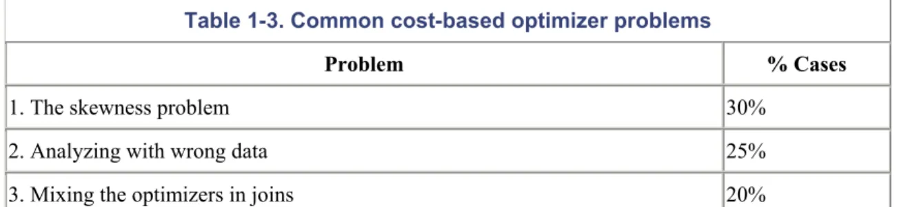
recommendation is that every site that is new to Oracle should be using the cost-based optimizer. I also recommend that sites currently using the rule-based optimizer have a plan in place for migrating to the cost-based optimizer. There are, however, some issues with the cost-based optimizer that you should be aware of. Table 1-3 lists the most common problems I have observed, along with their frequency of occurrence.
Table 1-3. Common cost-based optimizer problems
Problem % Cases
1. The skewness problem 30%
2. Analyzing with wrong data 25%
4. Choosing an inferior index 20%
5. Joining too many tables < 5%
6. Incorrect INIT.ORA parameter settings < 5%
1.4.1 Problem 1: The Skewness Problem
Imagine that we are consulting at a site with a table TRANS that has a column called STATUS. The column has two possible values: `O' for Open Transactions that have not been posted, and `C' for closed transactions that have already been posted and that require no further action. There are over one million rows that have a status of `C', but only 100 rows that have a status of `O' at any point in time.
The site has the following SQL statement that runs many hundreds of times daily. The response time is dismal, and we have been called in to "make it go faster."
SELECT acct_no, customer, product, trans_date, amt
FROM trans
WHERE status='O';
Response time = 16.308 seconds
In this example, taken from a real-life client of mine, the cost-based optimizer decides that Oracle should perform a full table scan. This is because the cost-based optimizer is aware of how many distinct values there are for the status column, but is unaware of how many rows exist for each of those values. Consequently, the optimizer assumes a 50/50 spread of data for each of the two values, `O' and `C'. Given this assumption, Oracle has decided to perform a full table scan to retrieve open transactions.
If we inform Oracle of the data skewness by specifying the option FOR ALL INDEXED
COLUMNS when we run the ANALYZE command or when we invoke the DBMS_STATS package, Oracle will be made aware of the skewness of the data; that is, the number of rows that exist for each value for each indexed column. In our scenario, the STATUS column is indexed. The following command is used to analyze the table:
After analyzing the table and computing statistics for all indexed columns, the cost-based optimizer is aware that there are only 100 or so rows with a status of `O', and it will accordingly use the index on that column. Use of the index on the STATUS column results in the following, much faster, query response:
Response Time: 0.259 seconds
Typically the cost-based optimizer will perform a full table scan if the value selected for a column has over 12% of the rows in the table, and will use the index if the value specified has less than 12% of the rows. The cost-based optimizer selections are not quite as firm as this, but as a rule of thumb this is the typical behavior that the cost-based optimizer will follow.
Prior to Oracle9i, if a statement has been written to use bind variables, problems can still occur with respect to skewness even if you use FOR ALL INDEXED COLUMNS. Consider the following example:
local_status := 'O';
SELECT acct_no, customer, product, trans_date, amt
FROM trans
WHERE status= local_status;
# Response time = 16.608
Notice that the response time is similar to that experienced when the FOR ALL INDEXED columns option was not used. The problem here is that the cost-based optimizer isn't aware of the value of the bind variable when it generates an execution plan. As a general rule, to overcome the skewness problem, you should do the following:
• Hardcode literals if possible. For example, use WHERE STATUS = `O', not WHERE STATUS = local_status.
• Always analyze with the option FOR ALL INDEXED COLUMNS.
ANALYZE INDEX
TRANS_STATUS_NDX
DELETE STATISTICS
Deleting the index statistics works because it forces rule-based optimizer behavior, which will always use the existing indexes (as opposed to doing full table scans).
Oracle9i will evaluate the bind variable value prior to deciding the execution plan, obviating the need to hardcode literal values.
1.4.2 Problem 2: Analyzing with Wrong Data
I have been invited to many, many sites that have performance problems at which I quickly determined that the tables and indexes were not analyzed at a time when they contained typical volumes of data. The cost-based optimizer requires accurate information, including accurate data volumes, to have any chance of creating efficient execution plans.
The times when the statistics are most likely to be forgotten or out of date are when a table is rebuilt or moved, an index is added, or a new environment is created. For example, a DBA might forget to regenerate statistics after migrating a database schema to a production environment. Other problems typically occur when the DBA does not have a solid knowledge of the database that he/she is dealing with and analyzes a table when it has zero rows, instead of when it has hundreds of thousands of rows shortly afterwards.
1.4.2.1 How to check the last analyzed date
To observe which tables, indexes, and partitions have been analyzed, and when they were last analyzed, you can select the LAST_ANALYZED column from the various user_XXX view. For example, to determine the last analyzed date for all your tables:
SELECT table_name, num_rows,
last_analyzed
FROM user_tables;
SELECT table_name
FROM all_tab_columns
WHERE column_name = 'LAST_ANALYZED'
This is not to say that you should be analyzing with the COMPUTE option as often as possible. Analyzing frequently can cause a tuned SQL statement to become untuned.
1.4.2.2 When to analyze
Re-analyzing tables and indexes can be almost as dangerous as adjusting your indexing, and should ideally be tested in a copy of the production database prior to being applied to the production database.
Peoplesoft software is one example of an application that uses temporary holding tables, with the table names typically ending with _TMP. When batch processing commences, each holding table will usually have zero rows. As each stage of the batch process completes, insertions and updates are happening against the holding tables.
The final stages of the batch processing populate the major Peoplesoft transaction tables by extracting data from the holding tables. When a batch run completes, all rows are usually deleted from the holding tables. Transactions against the holding tables are not committed until the end of a batch run, when there are no rows left in the table.
When you run ANALYZE on the temporary holding tables, they will usually have zero rows. When the cost-based optimizer sees zero rows, it immediately considers full table scans and Cartesian joins. To overcome this issue, I suggest that you populate the holding tables, and analyze them with data in them. You can then truncate the tables and commence normal processing. When you truncate a table, the statistics are not removed.
You can find INSERT and UPDATE SQL statements to use in populating the holding tables by tracing the batch process that usually populates and updates the tables. You can use the same SQL to populate the tables.
The runtimes of the batch jobs at one large Peoplesoft site in Australia went from over 36 hours down to under 30 minutes using this approach.
tables to use rule-based optimizer behavior. You can delete statistics using the ANALYZE TABLE
tname DELETE STATISTICS command. If the statistics are removed, it is important that you not allow the tables to join with tables that have valid statistics. It is also important that indexes that have statistics are not used to resolve any queries against the unanalyzed tables. If the temporary tables are used in isolation, and only joined with each other, the rule-based behavior is often preferable to that of the cost-based optimizer.
1.4.3 Problem 3: Mixing the Optimizers in Joins
As mentioned in the previous section, when tables are being joined, and one table in the join is analyzed and the other tables are not, the cost-based optimizer performs at its worst.
When you analyze your tables and indexes using the DBMS_STATS.GATHER_SCHEMA_STATS procedure and the GATHER_TABLE_STATS procedures, be careful to include the
CASCADE>=TRUE option. By default, the DBMS_STATS package will gather statistics for tables only. Having statistics on the tables, and not on their indexes, can also cause the cost-based
optimizer to make poor execution plan decisions.
One example of this problem that I experienced recently was at a site that had a TRANS table not analyzed, and an ACCT table analyzed. The DBA had rebuilt the TRANS table to purge data, and had simply forgotten to do the analyze afterwards. The following example shows the performance of a query joining the two tables:
SELECT a.account_name, sum(b.amount)
FROM trans b, acct a
WHERE b.trans_date > sysdate - 7
AND a.acct_id = b.acct_ID
AND a.acct_status = 'A'
GROUP BY account_name;
SORT GROUP BY
NESTED LOOPS
Response Time = 410 seconds
After the TRANS table was analyzed using the following command, the response time for the query was reduced by a large margin:
ANALYZE TABLE trans ESTIMATE STATISTICS
SAMPLE 3 PERCENT
FOR ALL INDEXED COLUMNS
The new execution plan, and response time, were as follows:
SORT GROUP BY
NESTED LOOPS
TABLE ACCESS BY ROWID ACCT
INDEX UNIQUE SCAN ACCT_PK
TABLE ACCESS BY ROWID TRANS
INDEX RANGE SCAN TRANS_NDX1
Response Time = 3.1 seconds
One other site that I was asked to tune had been instructed by the vendor of their personnel package to ANALYZE only their indexes and not their tables. The software provider had developed the software for Microsoft's SQL Server database, and had ported it to Oracle. The results of just analyzing the indexes caused widespread devastation. For example:
SELECT count(*)
FROM trans
WHERE acct_id = 9
AND cost_center = 'VIC';
TRANS_IDX2 is on ACCT_ID
TRANS_NDX3 is on COST_CENTER
Ironically, the software developers were blaming Oracle, claiming that it had inferior performance to SQL Server. After analyzing the tables and indexes, the response time of this SQL statement was dramatically improved to 0.415 seconds. The response times for many, many other SQL statements were also dramatically improved.
The moral of this story could be to let Oracle tuning experts tune Oracle and have SQL Server experts stick to SQL Server. However, with ever more mobile and cross-database trained IT professionals, I would suggest that we all take more care in reading the manuals when we tackle the tuning of a new database.
1.4.4 Problem 4: Choosing an Inferior Index
The cost-based optimizer will sometimes choose an inferior index, despite it appearing obvious that another index should be used. Consider the following Peoplesoft WHERE clause:
where
business_unit =
:5
and
ledger =
:6
and
fiscal_year =
:7
and
accounting_period =
:8
and
affiliate =
:9
and
statistics_code =
:10
and
project_id =
:11
and
account =
:12
and
currency_cd =
:13
and
deptid =
:14
and
product =
:15
The Peoplesoft system from which I took this example had an index that had every single column in the WHERE clause contained within it. It would seem that Oracle would definitely use that index when executing the query. Instead, the cost-based optimizer decided to use an index on
(BUSINESS_UNIT, LEDGER, FISCAL_YEAR, ACCOUNT). We extracted the SQL statement and compared its runtime to that when using a hint to force the use of the larger index. The runtime when using the index containing all the columns was over four times faster than the runtime obtained when using the index chosen by the cost-based optimizer.
When the index was rebuilt as a unique index, the index was used. The users were obviously happy with their four-fold performance improvement.
However, more headaches were to come. The same index was the ideal candidate for the following statement, which was one of the statements run frequently during end-of-month and end-of-year processing:
where
business_unit =
:5
and
ledger =
:6
and
fiscal_year =
:7
and
accounting_period between 1 and 12
and
affiliate =
:9
and
statistics_code =
:10
and
project_id =
:11
and
account =
:12
and
currency_cd =
:13
and
deptid =
:14
and
product =
:15
Despite the index being correctly created as UNIQUE, the cost-based optimizer was once again ignoring it. The only difference between this statement and the last is that this statement is after a
range of accounting periods for the financial year rather than just one accounting period.
This WHERE clause used the same incorrect index as previously mentioned, with the columns (BUSINESS_UNIT, LEDGER, FISCAL_YEAR, and ACCOUNT). Once again, we timed the statement using the index selected by the cost-based optimizer against the index that contained all of the columns, and found the larger index to be at least three times faster.
The problem was overcome by repositioning the ACCOUNTING_PERIOD column (originally third in the index) to be last in the index. The new index order was as follows:
business_unit
ledger
fiscal_year
affiliate
currency_cd
deptid
Product
accounting_period
Another way to force the cost-based optimizer to use an index is to use one of the hints that allows you to specify an index. This is fine, but often sites are using third-party packages that can't be modified, and consequently hints can't be utilized. However, there may be the potential to create a view that contains a hint, with users then accessing the view. A view is useful if the SQL that is performing badly is from a report or online inquiry that is able to read from views.
As a last resort, I have discovered that sometimes, to force the use of an index, you can delete the statistics on the index. Occasionally you can also ANALYZE ESTIMATE with just the basic 1,064 rows being analyzed. Often, the execution plan will change to just the way you want it, but this type of practice is approaching black magic. It is critical that if you adopt such a black magic approach, you clearly document what you have done to improve performance. Yet another method to try is lowering the OPTIMIZER_INDEX_COST_ADJ parameter to between 10 and 50.
In summary, why does the cost-based optimizer make such poor decisions? First of all, I must point out that poor decision-making is the exception rather than the rule. The examples in this section indicate that columns are looked at individually rather than as a group. If they were looked at as a group, the cost-based optimizer would have realized in the first example that each row looked at was unique without the DBA having to rebuild the index as unique. The second example illustrates that if several of the columns in an index have a low number of distinct values, and the SQL is requesting most of those values, the cost-based optimizer will often bypass the index. This happens despite the fact that collectively, the columns are very specific and will return very few rows.
In fairness to the optimizer, queries using indexes with fewer columns will often perform substantially faster than those using an index with many columns.
1.4.5 Problem 5: Joining Too Many Tables
Figure 1-1. A join of seven tables
The query expects to return just a handful of rows from the various tables, and the response time should be no longer than one second. Ideally, Oracle receives the ACCT_ADDRESS rows for the relevant account, and then joins to the ADDRESS table to determine if the addresses are in Washington.
However, because so many tables are being joined, the cost-based optimizer will often process F and G independently of the other tables and then merge the data at the end. The result of joining F and G first is that all address that are in the state of Washington must be selected. That process could take several minutes, causing the overall runtime to be far beyond what it would have been if Oracle had driven all table accesses from the A table.
Assuming you have an ACCT_ID index on the ACCT_ADDRESS (F) table, you can often
overcome this problem by placing a hint to tell the cost-based optimizer to use that index. This will speed the performance significantly.
Interestingly, the rule-based optimizer often makes a bigger mess of the execution plan when many tables are joined than does the cost-based optimizer. The rule-based optimizer often will not use the ACCT table as the driving table. To assist the rule-based optimizer, place the A table last in the FROM clause.
If you are using a third-party package, your best option may be to create a view with a hint, if that is allowable and possible with the package you are using.
1.4.6 Problem 6: Incorrect INIT.ORA Parameter Settings
When DBAs test changes in pre-production, they may work fine, but have problems with a different execution plan being used in production. How can this be? The reason for a different execution plan in production is often that there are different parameter settings in the production INIT.ORA file than in the pre-production INIT.ORA file.
I was at one site that ran the following update command and got a four-minute response, despite the fact that the statement's WHERE clause condition referenced the table's primary key. Oddly, if we
selected from the ACCT table rather than updating it, using the same WHERE clause, the index was
used.
UPDATE acct SET proc_flag = 'Y'
WHERE pkey=100;
# Response Time took 4 minutes and
# wouldn't use the primary key
We tried re-analyzing the table every which way, and eventually removed the statistics. The
statement performed well when the statistics were removed and the rule-based optimizer was used.
After much investigation, we decided to check the INIT.ORA parameters. We discovered that the COMPATIBLE parameter was set to 8.0.0 despite the database version being Oracle 8.1.7. We decided to set COMPATIBLE to 8.1.7, and, to our delight, the UPDATE statement correctly used the index and ran in about 0.1 seconds.
COMPATIBLE is not the only parameter that needs to be set the same in pre-production as in production to ensure that the cost-based optimizer makes consistent decisions. Other parameters include the following:
SORT_AREA_SIZE
The number of bytes allocated on a per-user session basis to sort data in memory. If the parameter is set at its default of 64K, NESTED LOOPS will be favored instead of SORT MERGES and HASH JOINS.
HASH_AREA_SIZE
The number of bytes to use on a per-user basis to perform hash joins in memory. The default is twice the SORT_AREA_SIZE. Hash joins often will not work unless this parameter is set to at least 1 megabyte.
Enables or disables the usage of hash joins. It has a default of TRUE, and usually doesn't need to be set.
OPTIMIZER_MODE
May be CHOOSE, FIRST_ROWS, or ALL_ROWS. CHOOSE causes the cost-based optimizer to be used if statistics exist. FIRST_ROWS will operate the same way, but will tend to favor NESTED LOOPS instead of SORT MERGE or HASH JOINS. ALL_ROWS will favor SORT MERGEs and HASH JOINS in preference to NESTED LOOP joins. DB_FILE_MULTIBLOCK_READ_COUNT
The number of blocks that Oracle will retrieve with each read of the table. If you specify a large value, such as 16 or 32, Oracle will, in many cases, bias towards FULL TABLE SCANS instead of NESTED LOOPS.
OPTIMIZER_MODE_ENABLE
Enables new optimizer features to be enabled. For example, setting the parameter to 8.1.7 will enable all of the optimizer features up to and including Oracle 8.1.7. This parameter can also automatically enable other parameters such as FAST_FULL_SCAN_ENABLED. Some of the major improvements that have occurred with the various Oracle versions include: 8.0.4 (ordered nested loops, fast full scans), 8.0.5 (many, many optimizer bug fixes), 8.1.6 (improved histograms, partitions, and nested loop processing), 8.1.7 (improved
partition handling and subexpression optimization), and 9.0.1 (much improved index joins, complex view merging, bitmap improvements, subquery improvements, and push join predicate improvements).
OPTIMIZER_INDEX_CACHING
Tells Oracle the percentage of index data that is expected to be found in memory. This parameter defaults to 0, with a range of 0 to 100. The higher the value, the more likely that NESTED LOOPS will be used in preference to SORT MERGE and HASH JOINs. Some sites have reported performance improvements when this parameter is set to 90. OPTIMIZER_INDEX_COST_ADJ
This parameter can be set to encourage the use of indexes. It has a default of 100. If you lower the parameter to 10, you are telling the cost-based optimizer to lower the cost of index usage to 10% of its usual value. You can also set the value to something way beyond 100 to force a SORT MERGE or a HASH JOIN. Sites report performance improvements when the parameter is set to between 10 and 50 for OLTP and 50 for decision support systems. Adjusting it downwards may speed up some OLTP enquiries, but make overnight jobs run forever. If you increase its value, the reverse may occur.
Causes a star transformation to be used to combine bitmap indexes on fact table columns. This is different from the Cartesian join that usually occurs for star queries.
QUERY_REWRITE_ENABLED
Allows the use of function-based indexes as well as allowing query rewrites for materialized views. The default is FALSE, which may explain why your function indexes are not being used. Set it to TRUE.
PARTITION_VIEW_ENABLED
Enables the use of partition views. If you are utilizing partitioned views, you will have to set this parameter to TRUE because the default is FALSE. A partition view is basically a view that has a UNION ALL join of tables. Partition views were the predecessor to Oracle partitions, and are used very successfully by many sites for archiving and to speed performance.
PARALLEL_BROADCAST_ENABLED
This parameter is used by parallel query when small lookup tables are involved. It has a default of FALSE. If set to TRUE, the rows of small tables are sent to each slave process to speed MERGE JOIN and HASH JOIN times when joining a small table to a larger table. OPTIMIZER_MAX_PERMUTATIONS
Can be used to reduce parse times. However, reducing the permutations can cause an inefficient execution plan, so this parameter should not be modified from its default setting. CURSOR_SHARING
If set to FORCE or SIMILAR, can result in faster parsing, reduced memory usage in the shared pool, and reduced latch contention. This is achieved by translating similar statements that contain literals in the WHERE clause into statements that have bind variables.
The default is EXACT. We suggest that you consider setting this parameter to SIMILAR with Oracle9ionly if you are certain that there are lots of similar statements with the only differences between them being the values in the literals. It is far better to write your application to use bind variables if you can.
Setting the parameter to FORCE causes the similar statements to use the same SQL area, which can degrade performance. FORCE should not be used.
Note that STAR TRANSFORMATION will not work if this parameter is set to SIMILAR or FORCE.
ALWAYS_SEMI_JOIN
STANDARD, which means that the main query (not the subquery) drives the execution plan. If you specifically set this parameter, the subquery becomes the driving query.
ALWAYS_ANTI_JOIN
This parameter will change the behavior of NOT IN statements, and can speed processing considerably if set to HASH or MERGE. Setting the parameter causes a merge or hash join rather than the ugly and time-consuming Cartesian join that will occur with standard NOT IN execution.
Remember that if any of these parameters are different in your pre-production database than in your production database, it is possible that the execution plans for your SQL statements will be different. Make the parameters identical to ensure consistent behavior.
1.5 Problems Common to Rule and Cost with Solutions
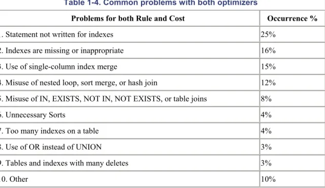
This section lists problems that are common to both the rule-based and cost-based optimizers. It is important that you are aware of these problems and avoid them wherever possible. Table 1-4 lists the problems and their occurrence rates.
Table 1-4. Common problems with both optimizers
Problems for both Rule and Cost Occurrence %
1. Statement not written for indexes 25%
2. Indexes are missing or inappropriate 16%
3. Use of single-column index merge 15%
4. Misuse of nested loop, sort merge, or hash join 12%
5. Misuse of IN, EXISTS, NOT IN, NOT EXISTS, or table joins 8%
6. Unnecessary Sorts 4%
7. Too many indexes on a table 4%
8. Use of OR instead of UNION 3%
9. Tables and indexes with many deletes 3%
10. Other 10%
Some SELECT statement WHERE clauses do not use indexes at all. Most such problems are caused by having a function on an indexed column. Oracle8i and later allow function-based indexes, which may provide an alternative method of using an effective index.
In the examples in this section, for each clause that cannot use an index, I have suggested an alternative approach that will allow you to get better performance out of your SQL statements.
In the following example, the SUBSTR function disables the index when it is used over an indexed column.
Do not use:
SELECT account_name, trans_date, amount
FROM transaction
WHERE
SUBSTR(account_name,1,7)
= 'CAPITAL';
Use:
SELECT account_name, trans_date, amount
FROM transaction
WHERE account_name
LIKE 'CAPITAL%'
;
In the following example, the!= (not equal) function cannot use an index. Remember that indexes can tell you what is in a table but not what is not in a table. All references to NOT, !=, and <>
disable index usage.
Do not use:
SELECT account_name,trans_date,amount
FROM transaction
WHERE amount
!= 0;
Use:
SELECT account_name,trans_date,amount
FROM transaction
WHERE amount
> 0
;
Do not use:
SELECT account_name, trans_date, amount
FROM transaction
WHERE
TRUNC(trans_date)
= TRUNC(SYSDATE);
Use:
SELECT account_name, trans_date, amount
FROM transaction
WHERE trans_date BETWEEN TRUNC(SYSDATE)
AND TRUNC(SYSDATE) + .99999;
In the following example, || is the concatenate function; it strings two character columns together. Like other functions, it disables indexes.
Do not use:
SELECT account_name, trans_date, amount
FROM transaction
WHERE account_name || account_type = 'AMEXA';
Use:
SELECT account_name, trans_date, amount
FROM transaction
WHERE account_name ='
AMEX'
AND
account_type =
'A'
;
In the following example, the addition operator is also a function and disables the index. All the other arithmetic operators (-, *, and /) have the same effect.
Do not use:
SELECT account_name, trans_date, amount
FROM transaction
WHERE
amount + 3000
< 5000;
SELECT account_name, trans_date, amount
FROM transaction
WHERE
amount < 2000
;
In the following example, indexes will not be used when a column or columns appears on both sides of an operator. The result will be a full table scan.
Do not use:
SELECT account_name, trans_date, amount
FROM transaction
WHERE
account_name
= NVL(:acc_name,
account_name
);
Use:
SELECT account_name, trans_date, amount
FROM transaction
WHERE account_name LIKE NVL(:acc_name, '%');
As mentioned previously, function indexes can be used if the function in the WHERE clause represents the same function and column on which the function index was created. For function indexes to work, you must have the INIT.ORA parameter QUERY_REWRITE_ENABLED set to TRUE. You must also be using the cost-based analyzer. The statement in the following example uses a function index:
CREATE INDEX results_fn_ndx1 ON results(UPPER(owner))
SELECT count(*)
FROM results
WHERE UPPER(owner) = 'MR M A GURRY';
Execution Plan
---
0 SELECT STATEMENT Optimizer=CHOOSE (Cost=1
Card=1 Bytes=32)
1 0 SORT (AGGREGATE)
2 1 INDEX (RANGE SCAN) OF
(Cost=1 Card=1 Bytes=32)
Another common problem that causes indexes not to be used is when the column indexed is one datatype and the value in the WHERE clause is another data type. Oracle automatically performs a simple column type conversion, or casting, when it compares two columns of different types. Assume that EMP_TYPE is an indexed VARCHAR2 column:
SELECT . . .
FROM emp
WHERE emp_type = 123
Execution Plan
---
SELECT STATEMENT OPTIMIZER HINT: CHOOSE
TABLE ACCESS (FULL) OF 'EMP'
Because EMP_TYPE is a VARCHAR2 value, and the constant 123 is a numeric constant, Oracle will cast the VARCHAR2 value to a NUMBER value. This statement will actually be processed as:
SELECT . . .
FROM emp
WHERE
TO_NUMBER
(emp_type) = 123
The EXPLAIN PLAN utility cannot detect or identify casting problems; it simply assumes that all module bind variables are of the correct type. Programs that are not performing up to expectation may have a casting problem. The EXPLAIN PLAN output will report that the SQL statement is correctly using the index, but that won't necessarily be true.
1.5.2 Problem 2: Indexes Are Missing or Inappropriate
While it is important to use indexes to reduce response time, the use of indexes can often actually
lengthen response times considerably. The problem occurs when more than 10% of a table's rows are accessed using an index.
Another important aspect of indexes is that depending on their type and composition, an index can affect the execution plan of a SQL statement. This must be considered when adding or modifying indexes.
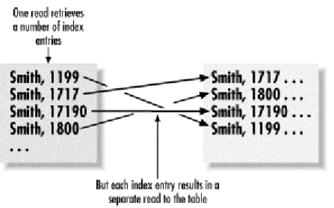
1.5.2.1 Indexing versus full table scans
Figure 1-2 depicts why an index may cause more physical reads than performing a FULL TABLE SCAN on an index. The table on the left side in Figure 1-2 shows the index entries with the
corresponding physical addresses on disk. The lines with the arrows depict physical reads from disk. Notice that each row accessed has a separate read.
Figure 1-2. Physical reads caused by an index
A full table scan is typically able to read over 100 rows of table information per block. Added to this, the DB_FILE_MULTIBLOCK_READ_COUNT parameter allows Oracle to read many blocks with one physical disk read. You may be reading 800 rows with each physical read from disk. In
comparison, an index will potentially perform one physical read for each row returned from the table.
If an index lookup is retrieving more than 10% of the rows in a table, the full table scan is likely to be a lot faster than index lookups followed by the additional physical reads to the table to retrieve the required data.
The exception to this rule is if the entire query can be satisfied by the index without the need to go to the table. In this case, an index lookup can be extremely effective. And if the SQL statement has an ORDER BY clause, and the index is ordered in the same order as the columns in the ORDER BY clause, a sort can be avoided, which can further improve performance.
In the following example, the runtime on the statement was reduced at a large stock brokerage from 40 seconds down to 3 seconds for account_id 100101, which happened to be the largest account in the table. The response time was critical for answering online customer inquiries. The problem was solved by adding all of the columns in the WHERE clause, and those in the SELECT list, into the index. There is the tradeoff that this index now has to be maintained, but the benefits at this site far outweighed the costs.
SELECT SUM(val)
FROM account_tran
WHERE account_id = 100101
AND