Molecular dynamics pre simulations for nanoscale computational fluid dynamics

Original citation:

Holland, David M., Lockerby, Duncan A., Borg, Matthew K., Nicholls, William D. and Reese,

Jason M.. (2015) Molecular dynamics pre-simulations for nanoscale computational fluid

dynamics. Microfluidics and Nanofluidics, 18 (3). pp. 461-474.

Permanent WRAP URL:

http://wrap.warwick.ac.uk/62574

Copyright and reuse:

The Warwick Research Archive Portal (WRAP) makes this work of researchers of the

University of Warwick available open access under the following conditions.

This article is made available under the Creative Commons Attribution 4.0 International

license (CC BY 4.0) and may be reused according to the conditions of the license. For more

details see:

http://creativecommons.org/licenses/by/4.0/

A note on versions:

The version presented in WRAP is the published version, or, version of record, and may be

cited as it appears here.

R E S E A R C H P A P E R

Molecular dynamics pre-simulations for nanoscale computational

fluid dynamics

David M. Holland•_{Duncan A. Lockerby}•

Matthew K. Borg•_{William D. Nicholls}•

Jason M. Reese

Received: 11 February 2014 / Accepted: 9 June 2014 / Published online: 20 June 2014 ÓThe Author(s) 2014. This article is published with open access at Springerlink.com

Abstract We present a procedure for using molecular

dynamics (MD) simulations to provide essential fluid and interface properties for subsequent use in computational fluid dynamics (CFD) calculations of nanoscale fluid flows. The MD pre-simulations enable us to obtain an equation of state, constitutive relations, and boundary conditions for any given fluid/solid combination, in a form that can be conveniently implemented within an otherwise conven-tional Navier–Stokes solver. Our results demonstrate that these enhanced CFD simulations are then capable of pro-viding good flow field results in a range of complex geometries at the nanoscale. Comparison for validation is with full-scale MD simulations here, but the computational cost of the enhanced CFD is negligible in comparison with the MD. Importantly, accurate predictions can be obtained in geometries that are more complex than the planar MD pre-simulation geometry that provides the nanoscale fluid properties. The robustness of the enhanced CFD is tested

by application to water flow along a (15,15) carbon nano-tube, and it is found that useful flow information can be obtained.

Keywords NanofluidicsComputational fluid dynamics

Molecular dynamicsHybrid methodsCarbon nanotubes

1 Introduction

Nanofluidic technologies are advancing rapidly, and a range of new technical opportunities are emerging, for example, efficient filtration of water using carbon nanotubes (CNT) (Alexiadis and Kassinos 2008; Mattia and Gogotsi 2008), heat removal and control in high heat-flux systems such as nuclear reactors, micro/nano-electro-mechanical systems (MEMS/NEMS), and micro-chemical reactors (Saidur et al.

2011; Wen et al.2009). However, the prediction of the fluid mass flow rate and heat transfer in nanoscale systems presents a major barrier to their design. The existence of non-contin-uum effects, such as molecular layering and velocity slip near to liquid–solid interfaces, seemingly precludes efficient con-tinuum computational fluid dynamics (CFD). On the other hand, more accurate molecular dynamics (MD) simulations can be extremely costly in terms of the computational resources they require. For example, to simulate 200 nm3 _of

water for 1 ns, with a modern MD code running on 8 CPUs in parallel, can require approximately 2 days of computational time. To simulate the liquid over much larger time and space scales is beyond the reach of current computational capabil-ities (even with the improved computational efficiency offered by graphical processing units, GPUs). This certainly prevents using such simulations within a practical iterative design process.

D. M. HollandD. A. Lockerby (&)

School of Engineering, University of Warwick, Coventry CV4 7AL, UK

e-mail: [email protected]

D. M. Holland

e-mail: [email protected]

M. K. BorgW. D. Nicholls

Department of Mechanical and Aerospace Engineering, University of Strathclyde, Glasgow G1 1XJ, UK e-mail: [email protected]

W. D. Nicholls

e-mail: [email protected]

J. M. Reese

School of Engineering, University of Edinburgh, Edinburgh EH9 3JL, UK

In this paper, we demonstrate that CFD simulations can still play a major role in nano-flow prediction for engi-neering design or, alternatively, for the initiation of steady-state MD simulations. We show that useful predictions can be readily and reliably obtained in complex nanoscale geometrical domains, despite the limits of the continuum-fluid assumption, if appropriate, continuum-fluid state models, vis-cosity relationships, and slip models are provided.

Both experiments and molecular simulations show that the continuum-fluid assumptions (e.g. local linear constitutive relationships) are still appropriate for water confined to channels of width *1–2 nm (see Bocquet and Charlaix (2010) and references therein), and MD simulations have been used to show that Lennard–Jones (LJ) fluids confined to geometries of *2–3 nm still show continuum behaviour (Huang et al.2007; Sofos et al.2009; Travis et al.1997). For nano-confined fluids below the continuum limit, however, the strain rate can vary rapidly within several molecular diame-ters (Todd et al. 2008) due to oscillations in the density; therefore, the stress becomes non-local. For quickly varying strain rates in homogeneous fluids, the non-local stress is calculable (Todd et al.2008), but for confined fluids, this is an unsolved problem [see for example Cadusch et al. (2008); Todd (2005)]. In addition, tests of continuum-fluid equation performance at the nanoscale have been restricted to extre-mely simple geometries, typically Poiseuille flow [e.g. Zhang et al. (2012)] and other canonical cases for which Hagen– Poiseuille equations are solved with slip boundary conditions. There is currently little substantive evidence to suggest that CFD can generally be applied at the nanoscale in arbitrary flow geometries.

In this paper, we make three contributions to nanofluidic modelling:

1. we propose a convenient pre-simulation MD frame-work that enables us to measure CFD-type properties (e.g. boundary conditions and constitutive relations) for a given solid/liquid combination;

2. we demonstrate that these fluid properties can be used to obtain highly accurate CFD predictions in complex geometries at the nanoscale, provided that a significant portion of the flow exhibits continuum bulk-like behaviour. This is distinct from previous studies [e.g. Zhang et al. (2012)] that focused mainly on 1D flow configurations. Importantly, we demonstrate that accurate CFD predictions can be obtained in cases that are more complex than the MD flow configuration from which the CFD fluid parameters were obtained; 3. we demonstrate that even in highly non-continuum 3D

flows, where no significant bulk flow exists (such as flow through some small diameter CNT), qualitatively accurate, and so useful, CFD predictions can be obtained.

The paper is structured as follows: in Sect.2, we define the MD procedure from which the fluid properties are extrac-ted for a particular liquid/solid combination. In Sect.3,this is applied to a LJ fluid interacting with solid bounding surface atoms that are effectively frozen. This is followed by nanoscale CFD predictions for three different geome-tries: a short channel connecting two reservoirs; a long channel connecting two reservoirs; and a channel with a geometrical irregularity connecting two reservoirs. The results in each case are compared with full MD data, which are vastly more computationally expensive and time-con-suming to obtain. In Sect.4, to demonstrate its applicability to highly non-continuum flows, we use our enhanced CFD to model water flow along a CNT. This example is chosen in order to explore the robustness of our approach for cases where the continuum assumption is known to be invalid. Finally, in Sect.5, we discuss the applications, limitations, and potential developments of the method.

2 Molecular dynamics procedure for generating fluid properties

We employ a preliminary MD simulation to obtain fluid properties and boundary conditions that enable the effec-tive use of a Navier–Stokes solver in nanoscale applica-tions it is typically not suitable for. This approach could be classed as a ‘sequential molecular-continuum hybrid method’ [see Mohamed and Mohamad (2010) for a review of hybrid methods], where ‘sequential’ refers to the fact that the MD is performed in advance of, and so indepen-dent of, the continuum model. In contrast, in ‘concurrent’ schemes, e.g. HMM (E et al.2009; Asproulis et al.2012) or Domain Decomposition (O’Connell and Thompson

1995), the MD simulations are fully coupled to a contin-uum model. While this is ultimately more likely to produce accurate solutions, it is certainly more computationally expensive. The sequential methodology we adopt instead is far more practical for preliminary and iterative engineering design simulations (at least, based on today’s computing capabilities). An example of a similar methodology can be found in Dongari et al. (2011a,b) in which molecular free path distributions within rarefied gases are measured using MD simulations and then used within the Navier–Stokes– Fourier equations.

paper, the atomic centres). The implications of the choice of the dependencies the fluid properties and boundary conditions on particular variables (here, density) are dis-cussed in Sect.5.

For efficiency and convenience, we propose a single MD configuration from which all of these fluid properties can be measured and/or controlled. This enables efficient concurrent MD simulations over any range of variables considered by multiple realisations of the same MD geometry/setup. We have chosen to use non-equilibrium MD (NEMD) simulations to gather the data rather than equilibrium MD despite potential, accuracy issues (Kan-nam et al. 2012), because this approach would be more suitable for simulating a complex fluid–solid interaction, where slip could be strain dependent. A possible more refined approach could be to use a combination of equi-librium MD simulations and NEMD simulations where appropriate.

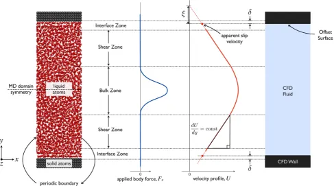
Figure1(far left) shows the MD pre-simulation domain; it is symmetrical about its centrelines and uses periodic boundary conditions in the streamwise direction (i.e. in the x-direction) and into the page (i.e. in thez-direction). The domain hasbulk,shearandinterfacezones (as labelled) for measuring state, constitutive and boundary properties, respectively. Pressure and density (and also temperature, if simulating non-isothermal cases) are measured in the bulk zone. In addition to this, in the bulk zone, an artificial

streamwise body force (Fx) is applied (see Fig. 1, centre left), which creates a velocity profile in the domain similar to that illustrated (centre right). We assume that the equation of state in the bulk zone is unaffected by the magnitude of strain rate generated. In the shear zone, the fluid is subject to a constant shear stress, sxy, directly resulting from the bulk-zone forcing. A linear flow velocity profile is developed in the shear zone, and this is least-squares fitted. The measured strain rate and shear stress are then used to obtain a viscosity coefficient,l, through

sxy ¼ ldU

dy: ð1Þ

In this paper, we assume that shear viscosity is sufficient to describe the fluid constitutive behaviour, while accepting that the pre-simulation configuration would need to be modified to deal with extensional viscosity.

Any significant density oscillations associated with molecular layering are confined to the interface zone. In this zone, we calculate what we term the ‘CFD surface displacement’ (d), which is the distance that a CFD wall/ surface needs to be displaced from the centres of surface atoms in order to accurately represent the boundary of the fluid (as opposed to the boundary of the solid); seedin Fig.

1. We take this displacement to be the distance from the centre of the surface wall atom to where the fluid density becomes at least 10 % of the bulk, i.e.qaqbulk, where

a¼0:1. The linear velocity profile obtained in the shear zone is extrapolated into the interface zone to find the apparent slip length, n, as defined from the CFD surface (see Fig.1, centre right).

Across multiple simulations, we obtain the bulk pres-sure, a viscosity coefficient, the slip length, and the surface displacement, for a range of combinations of bulk density and applied shear stress. In the MD simulations, the applied shear stress and bulk density are varied by modifying the body force and by adding/removing molecules, respec-tively, using the FADE algorithm (Borg et al. 2014). Finally, once all data are collected over the expected range of density and shear stress,1 functional relationships are constructed for the desired fluid properties (using, for example, fitted polynomials), which are then used in the CFD model. The behaviour of this CFD model ultimately depends on these functional relationships, and this choice requires some experience or needs to form part of an iterative approach (this is discussed in Sect. 5). For the cases considered in this paper, we adopt the following: for pressure,p¼pðqÞ; for dynamic viscosity,l¼lðqÞ; sur-face displacement,d¼dðqÞ; and slip length n¼nðq;c_Þ, whereqis the bulk fluid density andc_is the strain rate in the shear zone. This dependence on density would nor-mally imply a high-speed high-Mach number flow, but in nanoscale internal flows, it is possible to have substantial fluid compressibility at extremely low Mach numbers due to viscous-related pressure losses [see Gad-el Hak (2010) for a discussion of this]. For this reason, capturing the influence of density on fluid properties is critical to the accurate prediction of nanoscale flows. For all of the examples considered in this paper, the influence of strain rate can be safely ignored, but we consider its effect on slip length for demonstration purposes. The fluids we consider are therefore Newtonian in the bulk; a non-Newtonian fluid, for example, would at least requirel¼lðq;c_Þ. Note that for the simulation of well-understood fluids, it would not be necessary to extract all of these properties from MD pre-simulations.

3 CFD for nanoscale flow of a Lennard–Jones fluid

Owing to the lack of detailed and reliable experimental flow measurements at the nanoscale, in this section, we compare our enhanced CFD predictions with full-scale MD simula-tion results. This comparison is intended to test whether flow field solutions of comparable accuracy to full MD can be obtained from our enhanced CFD in complex nanoscale

geometries, without the need forad hoccorrections, and at only a fraction of the cost of full MD. A Lennard-Jones (LJ) model of liquid argon is chosen, where the solid wall atoms are fixed/frozen (Thompson and Troian 1997); the exact interatomic potentials used are given in ‘‘Appendix’’.

3.1 MD pre-simulation results

The MD pre-simulations are performed as described in Sect. 2, using the mdFoam solver (Borg et al. 2010; Macpherson et al.2007; Macpherson and Reese2008) that is implemented within the OpenFOAM libraries (Open-FOAM2013). The MD algorithm has molecules evolving using Newton’s equations of motion,midvi=dt¼fi, where

vi¼dri=dt;fi;ri and mi are the velocity, total force,

position and mass, respectively, of an arbitrary moleculei in a system ofN molecules at a timet. The total force per moleculefiis calculated at every time-step from the sum of

pair-wise intermolecular forces between molecules, i.e. fi¼P

N

j1 DU rij

for allj6¼i, whereUðrijÞis the potential energy when moleculesi andj are separated by rij¼ jrirjj.

The MD pre-simulation domain is constructed as illus-trated in Fig.1(far left) extending 4.08 nm and 5.44 nm in thex- andz-directions, respectively. These dimensions are principally chosen to be large enough to avoid unwanted ‘wrap-around’ effects due to the periodic boundaries. In the y-direction, each interface region extends by 0.68 nm, each shear zone extends by 3.4 nm, and the bulk zone extends by 4.08 nm, giving a total height of 12.24 nm. Owing to the symmetry of the problem, properties extracted from the shear and interface zones are mirrored and averaged (thus reducing the overall sampling time). The temperature is maintained at T=292.8 K by coupling molecules to a velocity-unbiased Berendsen thermostat (Berendsen et al.

1984) with a time constant of sT ¼21:6 fs, applied within 36 independent bins placed in they-direction, with each bin being 0.34 nm thick. It has been shown that using a ther-mostat on a confined fluid may affect the flow properties (Bernardi et al.2010); however, a thermostat is used in all the MD simulations in this work so that we can compare with isothermal CFD simulations. The same thermostat is used in both the pre-simulations and the full MD simula-tions; therefore, the same error is present in both—the verification of the simulation approach is thus not under-mined by any physical uncertainty introduced by the thermostat.

The pre-simulation is divided into two steps. In the first part of the simulation, the MD ensemble is set to the target density and allowed to run to a steady state (which takes

*1.5 million MD time-steps) with the external artificial force applied for the target strain rate. For any molecule in 1 _{In most cases, the expected ranges can be comfortably over}

the bulk region, the external forcing is given by a Gaussian distribution centred around the centreline of the simulation box:

FxðyÞ ¼Fexpðy2=2r2sÞn^x; ð2Þ

whereFis the magnitude of the Gaussian,rsis an estimate of the required width of the curve, andn^xis the unit vector in the x-direction. The relationship between the forcing magnitude and the shear stress can be obtained by substi-tuting Eq. (2) into the conservation of momentum and integrating giving:

F¼ 2sxy qnrs

ffiffiffiffiffiffi 2p

p : _ð3Þ

The second part of the pre-simulation is then used to measure the required fluid properties over an interval of around 2 million MD time-steps of 5.4 fs each.

3.1.1 Bulk pressure as a function of bulk density

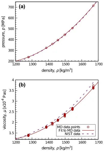
Figure 2a shows MD pre-simulation measurements of pressure, obtained from the standard Irving and Kirk-wood expression (1950), varying with the mass density.

The MD pre-simulation results are least-squares-fitted to a second-order polynomial. This then serves as an equation of state within the enhanced CFD solver to connect the mass continuity equation to the momentum equation. In this case, the polynomial is p¼0:001559q2_{3:387qþ2020:6. For reference, data}

from the NIST database for argon (Linstrom and Mal-lard 2001) are also plotted in Fig. 2a and is in close agreement with our MD pre-simulation data. Clearly, in this particular case, properties for argon are well known, but we extract the equation of state from our MD pre-simulation for the purposes of demonstration. The equation of state (and the viscosity equation in the following subsection) could be obtained by performing equilibrium MD simulations of a bulk fluid; however, the data are extracted from the pre-simulations here both for convenience and computational efficiency.

3.1.2 Dynamic viscosity as a function of density

The strain rate is extracted from the MD shear zone by a least-squares linear fit to the relaxed and time-averaged velocity profile. The applied shear stress is measured using the Irving–Kirkwood equation and then compared with the strain rate using Eq. (1) to give a dynamic shear viscosity coefficient for L-J argon at a given bulk density. The vis-cosity coefficients measured from our MD pre-simulations of LJ argon are shown in Fig. 2b. A least-squares poly-nomial fit of 2nd order in density is also plotted: l¼7:961010_q2_1:774106_{qþ0:001106. This is}

then used in our enhanced CFD simulations to close the momentum equation. Again, for reference, data from the NIST database for liquid argon are also plotted in Fig.2b. Note, due to the breakdown of the continuum assumption and the existence of non-local stress, this state-dependent viscosity becomes only approximate when applied to a nano-confined fluid.

3.1.3 CFD surface displacement as a function of density

The surface displacementddefines the location of the CFD boundaries relative to the atomic (actual) walls. Ifdvaries substantially with density (or any other fluid property), the geometry of the enhanced CFD domain becomes depen-dent on the CFD solution itself. However, for the fluid/ solid combinations considered in this paper, over the density ranges considered, d is effectively constant, see Fig. 3. This allows us to assume that the surface dis-placement is fixed, which avoids the need for a compli-cated recursive solution and re-meshing procedure. In previous work, the surface displacement has been set to the liquid–solid interaction length (Joseph and Aluru2008) or (a)

(b)

chosen in another arbitrary way, and in some cases neglected altogether. The liquid–solid interaction length is significantly larger than the surface displacement we pro-pose, which may be partly responsible for the large dis-crepancy between continuum-fluid predictions and MD results found in these previous studies, e.g. Joseph and Aluru (2008).

3.1.4 Slip length as a function of density and strain rate

Liquid slip velocity at surfaces is calculated using the Navier slip condition:

uslip ¼nc_; ð4Þ

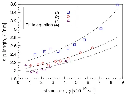
where n is the slip length and c_ is the shear rate at the bounding surface. The same least-squares-fitted linear velocity profile from Sect.3.1.2is used to calculate the slip length (as defined from the CFD surface). In this work, we only investigate steady isothermal liquid flows; therefore, our slip boundary condition only needs to depend on the strain rate [as in Thompson and Troian (1997)] and the density (Bocquet and Charlaix2010). In fact, the strain rate dependence is not necessary for the example cases we consider due to the relatively low shear rates, but here it is included for the purposes of illustration. Based on the strain rate/slip length relationship proposed in Thompson and Troian (1997), and assuming a linear dependence on den-sity, a least-squares fit is performed to the following equation:

n¼ðc1_{ffiffiffiffiffiffiffiffiffiffiffiffiffiffiffiffiffi}qþc2Þ

1c_=c_c

p ; _ð5Þ

where q is the density, c_c is the critical shear rate [see Thompson and Troian (1997)], and c1;c2 and c_ are

parameters of the fit to our MD pre-simulations, which are 1:20521012kg1m4;3:7468109m and 1:5431 1011s1, respectively. We leave the slip length dependence

on curvature [as discussed in Einzel et al. (1990)] for future refinement of this model.

Figure 4 shows our MD pre-simulation data and the least-squares fit of Eq. (5); results are shown for three different values of density. The slip model approximated by Eqs. (4) and (5) is directly introduced as a Robin boundary condition in the enhanced CFD solver. The slip length for the simple fluids modelled in this paper could be measured using equilibrium MD using similar methods to Bocquet and Barrat (1994); Hansen et al. (2011). However, for ease of application and generality (e.g. for capturing the interaction of solid surfaces with non-Newtonian fluids) we use this non-equilibrium methodology.

3.2 The enhanced CFD model

We perform finite-volume CFD simulations using Open-FOAM (2013), an open source set of C?? libraries for solving partial differential equations on unstructured meshes and in parallel. Specifically, we use the laminar, compressible solver sonicLiquidFoam, which we have modified to (a) accommodate a nonlinear equation of state, (b) allow a density-dependent viscosity, and (c) incorporate slip boundary conditions of the form given in Eq. (5). A compressible solver is used despite the very low Mach numbers, since, as dis-cussed above, significant compressibility can occur in micro-and nano-geometries (Gad-el Hak2010; Patronis et al.2013).

3.3 Simulation results

To test the reliability of our predictions using CFD enhanced with MD pre-simulation input, we compare them to results from full-domain MD calculations. We also compare results with predictions from compressible CFD with no-slip at the wall, and without modelling the CFD surface displacement

0.15 0.155 0.16 0.165 0.17 0.175 0.18 0.185 0.19 0.195 0.2

1300 1400 1500 1600 1700

surface displacement,

δ

[nm]

density, ρ [kg/m3] MD data points

Fig. 3 Surface displacementdvarying with fluid densityq, measured from each MD pre-simulation

1.8 2 2.2 2.4 2.6 2.8 3 3.2 3.4 3.6

0 1 2 3 4 5 6 7 8 9

slip length,

ξ

[nm]

strain rate, γ [x10-10 s-1]

ρ1

ρ2

ρ3

Fit to equation (4)

(referred to as ‘no-slip CFD’). We also compare with incompressible CFD with the same slip model but no surface displacement (referred to below as ‘incomp. slip CFD’). As test cases, we choose flows that all exhibit non-continuum behaviour (e.g. slip at surfaces), but also contain a significant bulk-flow region, even within the smallest features of the geometry. In Sect. 4 we consider the quality of CFD pre-dictions in cases where such a bulk region does not exist.

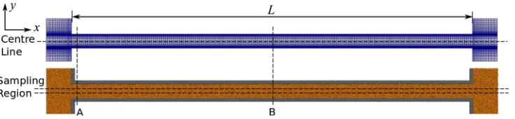
The two-dimensional cases we consider in this section involve connected reservoirs that are held at different pressures, an example of a filtration configuration, say. The first case has the reservoirs connected by a straight channel 108.8 nm long (Case 1), the second by a straight channel 231.2 nm long (Case 2), and the third by a 231.2 nm long straight channel with a cylindrical geometrical irregularity/ defect with radius 0.68 nm (Case 3). The channel width (measured as the distance between the centre of opposite solid surface atoms) is 4.08 nm for all three cases. Figure5

shows the CFD meshes for Case 1 alongside the corre-sponding full MD domain. Figure 6 shows the CFD and MD domain for Case 3 (L¼231:2 nm, with channel width of 4.08 nm; the width at the defect is 1.7 nm). For all three cases, the pressure at the inlet and outlet reservoir is 650 MPa and 300 MPa, respectively. The full MD simu-lations are used to evaluate the accuracy2of the enhanced

CFD predictions by comparison. As is standard CFD practice, the mesh resolution has been tested in each case to ensure mesh independence of the results.

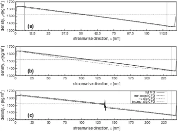
Figures 7a–c and 8a–c show results of pressure and density, respectively, along the centreline of each domain for each case. Both the centreline and the sampling region (where averaging is performed) are indicated on Fig.5. In Figs.7and8, differences between the CFD and MD results can be seen near the outermost boundaries of the reservoirs. This is because in the full-domain MD, for convenience, the reservoirs are connected by periodic boundary condi-tions, with a local body force imposing the pressure drop [see Docherty et al. (2014) for details of this approach]; in the CFD, however, boundary pressures can be specified directly, and so periodicity need not be enforced.

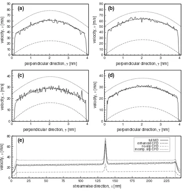
Velocity profiles cross-channel are presented in Fig.9a–d at cross sections A and B (as indicated on Fig.5) for Cases 1 and 2. The streamwise velocity along the centreline of the channel for Case 3 is presented in Fig.9e. Finally, in Table1, predictions for the mass flow rate through each channel are given.

In all three cases, the agreement between our enhanced CFD model (the dashed lines in Figs.7,8and9) and the MD results (solid lines) is extremely good for all of the flow variables considered. Also, CFD predictions of mass flow rate (arguably the most important bulk property in nano-channel flow cases, and one that no-slip CFD un-derpredicts very substantially) are all within 4 % of the

Fig. 6 Two-dimensional CFD and MD domains for Case 3 (top); close-up view of the channel irregularity (bottom) as an MD realisation (left) and a CFD mesh (right)

Fig. 5 Two-dimensional CFD mesh (top) and MD domain (bottom): Case 1,L¼108:8 nm; Case 2,L¼231:2 nm. Both channels are of width 4.08 nm

2 _{Strictly speaking, we mean ‘MD accuracy’ here, but for brevity we}

300 400 500 600 700

0 12.5 25 37.5 50 62.5 75 87.5 100 112.5

pressure,

p

[MP

a

]

streamwise direction,x[nm]

300 400 500 600 700

0 25 50 75 100 125 150 175 200 225

pressure,

p

[MP

a

]

streamwise direction,x[nm]

300 400 500 600 700

0 25 50 75 100 125 150 175 200 225

pressure,

p

[MPa

]

streamwise direction,x[nm]

full MD enhanced CFD no-slip CFD incomp. slip CFD

(c) (b) (a)

Fig. 7 Pressure along thecentrelineofaCase 1 (short channel),b Case 2 (long channel), andcCase 3 (defect channel). Thevertical linesatx¼6:8 nm andx¼115:6 nm (for Case 1) and atx¼6:8 nm and x¼238 nm (for Cases 2 and 3), indicate the inlet and outlet

positions, respectively. Full MD (solid line), enhanced CFD (dashed line), no-slip CFD (dash with dotted line) and incomp. slip CFD (dotted line)

1300 1400 1500 1600 1700

0 12.5 25 37.5 50 62.5 75 87.5 100 112.5

density,

[kg/m

3 ]

streamwise direction,x[nm]

1300 1400 1500 1600 1700

0 25 50 75 100 125 150 175 200 225

density,

[kg/m

3 ]

streamwise direction,x[nm]

1300 1400 1500 1600 1700

0 25 50 75 100 125 150 175 200 225

density,

[kg/m

3 ]

streamwise direction,x[nm] (a)

(b)

(c)

full MD enhanced CFD no-slip CFD incomp. slip CFD

Fig. 8 Density along the centreline of a) Case 1 (short channel), bCase 2 (long channel), andc) Case 3 (defect channel). Thevertical linesatx¼6:8 nm andx¼115:6 nm (for Case 1) and atx¼6:8 nm and x¼238 nm (for Cases 2 and 3), indicate the inlet and outlet

values obtained from full MD simulations. This very positive result is reassuring given the non-trivial nature of the geometry considered in Case 3, with the small non-planar irregularity in the channel. The MD simulation results show this small defect reduces the mass flow rate by more than 10 % (compared with the otherwise identical Case 2). Again, our enhanced CFD technique captures this effect accurately: the flow rate is reduced by 12 %.

Table2provides an indication of the computational cost for the three full-domain MD simulations. The longest simulations presented in this paper ran in parallel (on 24 CPUs) for 18 days. The laminar-flow CFD itself has a negligible cost by comparison, although the MD pre-sim-ulations also require the computational resources indicated in the last row of Table2. However, these pre-simulations need only to be performed once for a particular fluid/solid

0 10 20 30 40 50 60 70 80 90

0 1 2 3 4

ve

locity,

[m/

s

]

perpendicular direction,y[nm]

0 10 20 30 40 50 60 70 80 90

0 1 2 3 4

velocity,

[m/s]

perpendicular direction,y[nm]

0 10 20 30 40

0 1 2 3 4

ve

loci

ty,

[m/s]

perpendicular direction,y[nm]

0 10 20 30 40

0 1 2 3 4

velocity,

[m/s]

perpendicular direction,y[nm] (b)

(a)

(d) (c)

0 20 40 60 80

0 25 50 75 100 125 150 175 200 225

vel

oc

ity,

[m/s]

streamwise direction,x[nm]

(e) full MD

enhanced CFD no-slip CFD incomp. slip CFD

Fig. 9 Streamwise velocity profiles foraCase 1 at section A;bCase 1 at section B;c) Case 2 at section A; dCase 2 at section B; and eCase 3 along thecentreline. Thevertical linesatx¼6:8 nm and

x¼238 nm in (e) represent the inlet and outlet, respectively. Full MD (solid line), enhanced CFD (dashed line), no-slip CFD (dash with dotted line) and incomp. slip CFD (dotted line)

Table 1 Mass flow rate predictions (per unit length, because of the 2D geometry) for each channel case and model

Full MD

_

mmd104½kg/m/s

Enhanced CFD

_

mA104½kg/m/s (%)

No-slip CFD

_

mB104½kg/m/s(%)

Incomp. slip CFD

_

mC104½kg/m/s(%)

Short Channel 3.25 3.18 (-2.3) 1.13 (-65) 4.21 (?29)

Long Channel 1.57 1.51 (-3.7) 0.53 (-66) 2.09 (?33)

Defect Channel 1.32 1.35 (?2.2) 0.49 (-63) 1.87 (?41)

combination and then used for any number of flow geometries thereafter.

4 Water flow through carbon nanotube (CNT) membranes

In this section, we test the robustness of our enhanced CFD technique for cases where, in some region of the flow field, the continuum-fluid assumption is far from being valid, and where there also exist large regions of bulk fluid for which MD is prohibitively expensive. The three-dimensional flow configuration we consider is essentially the same as depicted in Fig.5, except that the two reservoirs of water, held at different pressures, are now separated by a (15,15) CNT of length 50 nm and diameter approximately 2 nm; since the domain is periodic in the y- and z-directions, this setup represents a regularly repeated array of CNTs. The flow of water through CNTs has recently been the focus of substantial research effort (Alexiadis and Kassinos 2008) mainly due to the extremely high flow rates that have been both predicted (Nicholls et al.2012) and measured (Mattia and Gogotsi2008; Whitby and Quirke 2007). These flow rates are often expressed as an enhancement factor, which is the ratio of water flow rates along the CNT to those predicted by classical fluid dynamics (i.e. the Hagen– Poiseuille equation). The low friction associated with this

water transport, and the high selectivity of CNTs, makes CNTs (and other nanotubes) excellent candidates for high-efficiency desalination and other filtration applications. The high flow rates, often reported as being orders of magnitude greater than classical flow theory predicts (Whitby and Quirke 2007), are typically attributed to both weak sur-face–fluid interactions and molecular ordering/layering that enables water molecules to pass efficiently along the CNT in a semi-ordered or structured manner.

Clearly, this kind of flow is difficult to describe accu-rately with a continuum-fluid model, but we demonstrate below that reasonable results can still be obtained for some spatially and temporally averaged properties. The likely reason that our enhanced CFD estimates are reasonable is that the flow in the CNT is dictated by the liquid interaction with the smooth graphitic surface (which is adequately modelled), despite the non-continuum conditions within the fluid.

4.1 MD pre-simulation results

The MD pre-simulations for this case are constructed identically to these of Sect.3, including the dimensions of the geometry. Here, though, the TIP4P/2005 molecular water model is used to describe the condensed phase of water, while the solid boundary walls consist of atom-thick graphene sheets that are modelled using 663 frozen carbon atoms. The exact interatomic potentials used are given in ‘‘

Appendix’’. As water is a well-known fluid, we use data from NIST (Linstrom and Mallard2001) for the pressure– density and density–viscosity relationships, both of which are fitted to quadratic polynomials. For the pressure–den-sity relationship, the equation used is p¼0:00684q2

11:49qþ4655, and for the density–viscosity relationship we use:l¼1:413108_q2:879105_qþ0:01555.

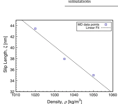
MD pre-simulations provide values for the surface displacement (i.e. from the carbon atoms to the fluid) and the slip length over the range of densities within the channel. As the strain rate is low, we only use three data points to model a linear dependency of the slip length on density, i.e.

n¼c1qþc2; ð6Þ

Table 2 Computational costs: the first three rows are the full MD simulations, while the last row is the MD pre-simulation that is used to collect the data for the enhanced CFD

CPUs Liquid molecules

Wall molecules

Time per MD time-step (s)

Total computational time

Short Channel 24 89,146 133,424 0.7 10 days

Long Channel 24 162,084 275,280 1.3 18 days

Defect Channel

24 161,369 276,830 1.3 18 days

MD pre-simulations

24 5,073-6,668 4,160 0.14 4 days per liquid/solid combination

32 34 36 38 40 42 44

1010 1020 1030 1040 1050 1060

Slip Length,

ξ

[nm]

Density, ρ [kg/m3_]

MD data points Linear Fit

wherec1andc2are parameters of the fit and are2:8248

1010kg1m4 and 3:3117107nm, respectively. In this case, for the enhanced CFD simulations we take d¼ 0:266 nm and the slip length relationship is shown in Fig.10.

4.2 Simulation results

We again compare our enhanced CFD predictions against full MD results and against the standard CFD models

outlined in Sect. 3. The CFD mesh is chosen to be fine enough to safely give mesh-independent results for mass flow rate; given that the cost of the CFD simulations is extremely small, achieving this poses no particular prob-lem. The pressure difference between the reservoirs is set to be 200 MPa because it is very challenging to obtain useful information from MD using only low pressure dif-ferences due to the extended sampling times required to filter low-velocity signals from the thermal noise (Nicholls et al. 2012). These high pressure (and consequently

850 900 950 1000 1050 1100 1150 1200

0 10 20 30 40 50 60

density,

[kg/m

3 ]

streamwise direction,x[nm]

-50 0 50 100 150 200 250

0 10 20 30 40 50 60

pressure,

p

[MPa]

streamwise direction,x[nm]

MD enhanced CFD no-slip CFD incomp. slip CFD (a)

(b)

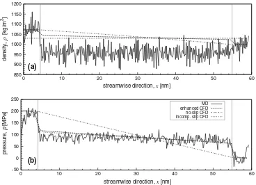
Fig. 11 Water density and pressure along thecentrelineof the CNT. The noise in the MD data is due to the relatively small number of molecules being sampled in the absence of a well defined ‘bulk-flow’ region. Thevertical linesatx¼4:4 nm andx¼55:8 nm represent the

inlet and outlet, respectively. Full MD (solid line), enhanced CFD (dashed line), no-slip CFD (dash with dotted line) and incomp. slip CFD (dotted line)

0 5 10 15 20 25 30

0 0.1 0.2 0.3 0.4 0.5 0.6 0.7 0.8 0.9 1

Velocity,

v

[m/s]

Normal distance to wall,d[nm] full MD enhanced CFD no-slip CFD incomp. slip CFD

0 500 1000 1500 2000 2500 3000

0 0.1 0.2 0.3 0.4 0.5 0.6 0.7 0.8 0.9 1

Density,

[kg/m

3]

Normal distance to wall,d[nm] full MD enhanced CFD pre-simulation MD

(a) (b)

density) differences make the CFD predictions even more challenging. The full MD simulation was performed in parallel on 48 CPUs, with the majority of the computa-tional effort attributable to the two reservoir regions. These have dimensions 4:410:610:3 nm and are chosen to be large enough to avoid any effects on the CNT flow due to reservoir boundaries. The intermolecular potentials used are the same as those in the pre-simulation, as given in ‘‘Appendix’’.

Figure 11 shows pressure and density plots along the centreline of the CNT; in the MD, this is done within a cylinder of radius 0.1577 nm about the centreline. Due to the substantial density fluctuations within the MD simula-tions (see Fig. 11b), a bulk density effectively does not exist, and the choice of the size of this sampling region can substantially affect the bulk density measured. The no-slip CFD model does not exhibit large pressure drops at the inlet and the outlet due to the much lower velocity in the tube (and therefore, there are lower accelerations at the inlet and outlet) than in the slip cases. Cross-sectional velocity profiles in the centre of the CNT are plotted in Fig.

12a. The mass flow rate in the full MD simulation is measured to be 4:31014kg/s, which is 23% greater than that predicted by our enhanced CFD. That this is a significant improvement on conventional CFD model pre-dictions is indicated in Table3.

Given the 2 nm diameter of the (15,15) CNT and despite the molecular layering that actually occurs within the flow field, as evidenced in Fig.12b, our enhanced CFD approach can be considered reasonably robust in predicting important averaged fluid properties to the correct order of magnitude. These CFD results are obtained with negligible cost in comparison with full MD simulations.

5 Discussion and conclusions

A new procedure for solving nanoscale flows using CFD has been presented. The state, constitutive, and boundary condition information for the CFD solver is extracted from MD pre-simulations. We have demonstrated that this enhanced solver can then provide good predictions for a range of nanoscale flow geometries. A number of questions and possibilities now arise. What happens when CFD is applied far beyond the limits of its applicability? For example, how robust is the predictive performance of CFD

at the nanoscale? These questions have been addressed, at least to some extent, by our results for water flow along a CNT. Our answer is CFD can be more robust than perhaps is often implied in the literature. A deeper investigation into how CFD and the continuum-fluid model perform at the limits of their applicability is needed; unfortunately, this may be restricted by the need to assess their accuracy by comparison with expensive MD simulations.

Another natural question relates to how these CFD simulations should be used given that, by comparison with MD, they are computationally cheap. It is not the case that CFD can replace MD for nanoscale simulations (in the same way that MD cannot replace experiment). However, there are a number of situations in which CFD enhanced with MD pre-simulations can be an invaluable affordable alternative or addition to MD. For example, in iterative conceptual design, where multiple simulations with slightly modified geometries are required; in initialising full-scale MD simulations, which would otherwise need to be sim-ulated for a much longer time in order for the flow to develop from a stationary to a steady state (Kalweit2008); and in helping to locate far-field and symmetry boundaries in full-scale MD simulations, such that their influence is not felt in the flow region of interest.

There is also the possibility that enhanced CFD could be used in some cases to produce more realistic predictions than MD. Quite often MD simulations are performed at much higher velocities (orders of magnitude higher) than would be seen in reality, solely for the purpose of increasing the signal to noise ratio (as is the case for the CNT simulations in Sect.4). These simulations rely on the assumption that the system behaves linearly up to the extreme condition. While a full MD simulation at realistic velocities is currently extremely challenging [although not intractable (Wang et al.2012)], a single MD pre-simulation for one fluid/solid combination is far less so. This would enable enhanced CFD to be used to investigate whether the linear response assumption is likely to be valid for a par-ticular configuration.

A criticism of this CFD approach is that it requires an assumption beforehand about the flow and fluid behaviour. For example, the viscosity coefficient for a fluid may depend on a multitude of fluid variables with a variety of functional forms; in the examples of this paper, we have assumed these functional forms based on our experience. This is true also of hybrid particle/continuum methods in

Table 3 Water mass flow rate predictions for each model of the CNT

Full MD (m_md1014kg/s) Enhanced CFD (m_A1014kg/s) No-slip CFD (m_B1014kg/s) Incomp. slip CFD (m_C1014kg/s)

CNT 4.3 3.3 (-23 %) 0.15 (-97 %) 9.0 (?109 %)

general and is not unique to the method we propose. The molecular-based simulations of HMM (Ren and E2005), for example, have to be ‘constrained’ by the overall con-tinuum model; the choice of how the constraint is per-formed (i.e. what variables are to be imposed on the MD subdomain) requires similar suppositions about how the fluid will behave. Also, in the present paper, we have assumed that the channels are homogeneously filled with fluid before the simulation begins. This neglects the multi-phase, transient problems that occur in the fill-up process of a CNT or the flow through nano-pores, such as an aqu-aporin. Currently, these types of problems could not be solved by our enhanced CFD.

An additional advantage of the approach in this paper is that it can be deployed recursively (and not neces-sarily for the same CFD simulation, or by the same researcher/designer). For example, a basic simula-tion could be used to make a first-estimate CFD pre-diction; subsequent MD simulations could then be used to refine and finesse the fluid and interface models, thereby producing successively more accurate CFD predictions. Users would need to approach this refine-ment and finessing of fluid property models for enhanced CFD in the same way as they would a con-ventional mesh-dependency study.

Acknowledgments This work is financially supported in the UK by EPSRC Programme Grant EP/I011927/1 and EPSRC Grants EP/ K038664/1 and EP/K038621/1. Our calculations were performed on the high-performance computer ARCHIE at the University of Strathclyde, funded by EPSRC Grants EP/K000586/1 and EP/K000195/1.

Open Access This article is distributed under the terms of the Creative Commons Attribution License which permits any use, dis-tribution, and reproduction in any medium, provided the original author(s) and the source are credited.

Appendix

MD intermolecular potentials for the Lennard–Jones cases

For the straight channel and defect channel simulations, we use a simple monatomic fluid with the LJ 6–12 potential with a cut-off radius:

ULJ rij ¼ 4e r12

r12

ij r

6

r6

ij

" #

ifrijrc;

0 ifrij[rc;

8 > < >

: ð7Þ

where r and are the length in the system and energy characteristics of the potential, andrc is the cut-off sepa-ration. The r and properties for the liquid-liquid and wall–liquid interactions are taken from Thompson and Troian (1997): rll¼3:41010m; ll¼1:657

1021J;rwl¼2:551010m; wl¼0:331021J and rc¼1:36 nm. The solid mass density is qw¼6:809103kg/m3, and the liquid mass density is ql¼1:431103kg/m

3_{, where the mass of one wall or}

liquid molecule is 6:69041026_{kg. The time-step in the}

MD simulations is 5.4 fs.

MD intermolecular potentials for the water in a CNT case

The rigid TIP4P/2005 water model (Abascal and Vega

2005; Huggins2012; Vega and Abascal2011) is used. This water model consists of four interacting sites: one oxygen atom (O) with no charge but which is the centre of the LJ potential, two hydrogen sites (H) each with a fixed point charge of qH¼0:5564e, and a massless site (M) with charge qM¼ 1:1128e. All oxygen atoms interact using the LJ potential, Eq. (7) withOO¼0:77491021J and rOO¼3:15891010m. Water–carbon interactions also use the LJ potential between carbon and oxygen atoms with rCO¼3:191010m andCO¼0:7093021021J as in Ritos et al. (2014). These values reproduce the macro-scopic contact angle of a water droplet on a graphitic surface, using the methodology of Werder et al. (2003). The other charged sites interact via the Coulomb potential:

UCðrijÞ ¼ 1 4p0

qiqj

rij ; ð8Þ

where qi;qj are the site charges and 0 is the vacuum

permittivity. To reduce computational time, this potential is shifted to be zero at rc¼1:0 nm:

UC rij ¼

UC rij UCð Þrc ifrijrc;

0 ifrijrc:

ð9Þ

The time-step for all MD water simulations is set to 2:16 fs.

References

Abascal JLF, Vega C (2005) A general purpose model for the condensed phases of water: TIP4P/2005. J Chem Phys 123(234):505

Alexiadis A, Kassinos S (2008) Molecular simulation of water in carbon nanotubes. Chem Rev 108(12):5014–5034

Asproulis N, Kalweit M, Drikakis D (2012) A hybrid molecular continuum method using point wise coupling. Adv Eng Softw 46(1):85–92

Berendsen H, Postma J, van Gunsteren W, DiNola A, Haak J (1984) Molecular dynamics with coupling to an external bath. J Chem Phys 81(8):3684–3690

Bernardi S, Todd B, Searles DJ (2010) Thermostating highly confined fluids. J Chem Phys 132(24):244,706

Bocquet L, Charlaix E (2010) Nanofluidics, from bulk to interfaces. Chem Soc Rev 39(3):1073–1095

Borg MK, Macpherson GB, Reese JM (2010) Controllers for imposing continuum-to-molecular boundary conditions in arbi-trary fluid flow geometries. Mol Simul 36(10):745–757 Borg MK, Lockerby DA, Reese JM (2014) The fade mass-stat: a

technique for inserting or deleting particles in molecular dynamics simulations. J Chem Phys, in press

Cadusch PJ, Todd B, Zhang J, Daivis PJ (2008) A non-local hydrodynamic model for the shear viscosity of confined fluids: analysis of a homogeneous kernel. J Phys A Math Theor 41(3):035,501

Docherty SY, Nicholls WD, Borg MK, Lockerby DA, Reese JM (2014) Boundary conditions for molecular dynamics simulations of water transport through nanotubes. Proc Inst Mech Eng Part C J Mech Eng Sci 228:186–195

Dongari N, Zhang Y, Reese JM (2011) Modeling of knudsen layer effects in micro/nanoscale gas flows. Trans ASME-I J Fluids Eng 133(7):071,101

Dongari N, Zhang Y, Reese JM (2011) Molecular free path distribution in rarefied gases. J Phys D Appl Phys 44(12):125,502

E W, Ren W, Vanden-Eijnden E (2009) A general strategy for designing seamless multiscale methods. J Comput Phys 228(15):5437–5453

Einzel D, Panzer P, Liu M (1990) Boundary condition for fluid flow: curved or rough surfaces. Phys Rev Lett 64(19):2269–2272 Gad-el Hak M (2010) MEMS: introduction and fundamentals. CRC

Press, Boca Raton

Hansen JS, Todd B, Daivis PJ (2011) Prediction of fluid velocity slip at solid surfaces. Phys Rev E 84(1):016,313

Huang C, Choi P, Nandakumar K, Kostiuk L (2007) Comparative study between continuum and atomistic approaches of liquid flow through a finite length cylindrical nanopore. J Chem Phys 126(22):224,702–224,702

Huggins DJ (2012) Correlations in liquid water for the TIP3P-Ewald, TIP4P-2005, TIP5P-Ewald, and SWM4-NDP models. J Chem Phys 136(064):518

Irving J, Kirkwood JG (1950) The statistical mechanical theory of transport processes. iv. The equations of hydrodynamics. J Chem Phys 18:817–829

Joseph S, Aluru N (2008) Why are carbon nanotubes fast transporters of water? Nano Lett 8(2):452–458

Kalweit M (2008) Molecular modelling of meso-and nanoscale dynamics. PhD thesis, Cranfield University.

Kannam SK, Todd B, Hansen JS, Daivis PJ (2012) Slip length of water on graphene: limitations of non-equilibrium molecular dynamics simulations. J Chem Phys 136(2):024,705

Linstrom PJ, Mallard WG (2001) NIST chemistry webbook; NIST standard reference database no. 69.http://webbook.nist.gov Macpherson GB, Reese JM (2008) Molecular dynamics in arbitrary

geometries: parallel evaluation of pair forces. Mol Simul 34(1):97–115

Macpherson GB, Borg MK, Reese JM (2007) Generation of initial molecular dynamics configurations in arbitrary geometries and in parallel. Mol Simul 33(15):1199–1212

Mattia D, Gogotsi Y (2008) Review: static and dynamic behavior of liquids inside carbon nanotubes. Microfluid Nanofluid 5(3):289–305

Mohamed KM, Mohamad AA (2010) A review of the development of hybrid atomistic–continuum methods for dense fluids. Microfluid Nanofluid 8(3):283–302

Nicholls WD, Borg MK, Lockerby DA, Reese JM (2012) Water transport through (7, 7) carbon nanotubes of different lengths using molecular dynamics. Microfluid Nanofluid 12(1–4):257–264

O’Connell ST, Thompson PA (1995) Molecular dynamics-continuum hybrid computations: a tool for studying complex fluid flows. Phys Rev E 52, pp. R5792–R5795. doi:10.1103/PhysRevE.52. R5792,http://link.aps.org/doi/10.1103/PhysRevE.52.R5792 OpenFOAM (2013) The open source CFD toolbox. http://www.

openfoam.org

Patronis A, Lockerby DA, Borg MK, Reese JM (2013) Hybrid continuum–molecular modelling of multiscale internal gas flows. J Comput Phys 255:558–571

Ren W, E W (2005) Heterogeneous multiscale method for the modeling of complex fluids and micro-fluidics. J Comput Phys 204(1):1–26. doi:10.1016/j.jcp.2004.10.001, http://www.science direct.com/science/article/pii/S0021999104004048

Ritos K, Mattia D, Calabr F, Reese JM (2014) Flow enhancement in nanotubes of different materials and lengths. J Chem Phys 140(1):014702. doi:10.1063/1.4846300, http://scitation.aip.org/ content/aip/journal/jcp/140/1/10.1063/1.4846300

Saidur R, Leong KY, Mohammad HA (2011) A review on applica-tions and challenges of nanofluids. Renew Sustain Energy Rev 15:1646–1668

Sofos F, Karakasidis T, Liakopoulos A (2009) Transport properties of liquid argon in krypton nanochannels: anisotropy and non-homogeneity introduced by the solid walls. Int J Heat Mass Transf 52(3–4):735–743

Thompson PA, Troian SM (1997) A general boundary condition for liquid flow at solid surfaces. Nature 389(6649), pp. 360–362. doi:10.1038/38686, http://www.nature.com/nature/journal/v389/ n6649/full/389360a0.html

Todd B (2005) Cats, maps and nanoflows: some recent developments in nonequilibrium nanofluidics. Mol Simul 31(6–7):411–428 Todd B, Hansen J, Daivis PJ (2008) Nonlocal shear stress for

homogeneous fluids. Phys Rev Lett 100(19):195,901

Travis KP, Todd BD, Evans DJ (1997) Departure from Navier–Stokes hydrodynamics in confined liquids. Phys Rev E 55(4):4288 Vega C, Abascal JLF (2011) Simulating water with rigid

non-polarizable models: a general perspective. Phys Chem Chem Phys 13(44):19,663–19,688

Wang L, Dumont RS, Dickson JM (2012) Nonequilibrium molecular dynamics simulation of water transport through carbon nanotube membranes at low pressure. J Chem Phys 137(044):102 Wen D, Lin G, Vafaei S, Zhang K (2009) Review of nanofluids for

heat transfer applications. Particuology 7(2):141–150

Werder T, Walther JH, Jaffe RL, Halicioglu T, Koumoutsakos P (2003) On the water–carbon interaction for use in molecular dynamics simulations of graphite and carbon nanotubes. J Phys Chem B 107(6):1345–1352

Whitby M, Quirke N (2007) Fluid flow in carbon nanotubes and nanopipes. Nat Nanotechnol 2(2):87–94