Linking long term planetary N body simulations with periodic orbits : application to white dwarf pollution

warwick.ac.uk/lib-publications

Original citation:

Antoniadou, Kyriaki I. and Veras, Dimitri. (2016) Linking long-term planetary N-body

simulations with periodic orbits : application to white dwarf pollution. Monthly Notices of

the Royal Astronomical Society, 463 (4). pp. 4108-4120.

Permanent WRAP URL:

http://wrap.warwick.ac.uk/81836

Copyright and reuse:

The Warwick Research Archive Portal (WRAP) makes this work by researchers of the

University of Warwick available open access under the following conditions. Copyright ©

and all moral rights to the version of the paper presented here belong to the individual

author(s) and/or other copyright owners. To the extent reasonable and practicable the

material made available in WRAP has been checked for eligibility before being made

available.

Copies of full items can be used for personal research or study, educational, or not-for profit

purposes without prior permission or charge. Provided that the authors, title and full

bibliographic details are credited, a hyperlink and/or URL is given for the original metadata

page and the content is not changed in any way.

Publisher’s statement:

This is a pre-copyedited, author-produced PDF of an article accepted for publication in

Monthly Notices of the Royal Astronomical Society following peer review. The version of

record Antoniadou, Kyriaki I. and Veras, Dimitri. (2016) Linking long-term planetary N-body

simulations with periodic orbits : application to white dwarf pollution. Monthly Notices of

the Royal Astronomical Society, 463 (4). pp. 4108-4120. is available online at:

http://dx.doi.org/10.1093/mnras/stw2264

A note on versions:

The version presented here may differ from the published version or, version of record, if

you wish to cite this item you are advised to consult the publisher’s version. Please see the

‘permanent WRAP url’ above for details on accessing the published version and note that

access may require a subscription.

Linking long-term planetary

N

-body simulations with

periodic orbits: application to white dwarf pollution

Kyriaki I. Antoniadou

, Dimitri Veras

1_{Department of Physics, Aristotle University of Thessaloniki, 54124 Thessaloniki, Greece}

2_{Department of Physics, University of Warwick, Coventry CV4 7AL, UK}

Accepted XXX. Received YYY; in original form ZZZ

ABSTRACT

Mounting discoveries of debris discs orbiting newly-formed stars and white dwarfs (WDs) showcase the importance of modeling the long-term evolution of small bodies in exosystems. WD debris discs are in particular thought to form from very long-term (0.1-5.0 Gyr) instability between planets and asteroids. However, the time-consuming nature ofN-body integrators which accurately simulate motion over Gyrs necessitates a judicious choice of initial conditions. The analytical tools known asperiodic orbitscan circumvent the guesswork. Here, we begin a comprehensive analysis directly linking periodic orbits with N-body integration outcomes with an extensive exploration of the planar circular restricted three-body problem (CRTBP) with an outer planet and inner asteroid near or inside of the 2:1 mean motion resonance. We run nearly 1000 focused simulations for the entire age of the Universe (14 Gyr) with initial conditions mapped to the phase space locations surrounding the unstable and stable periodic orbits for that commensurability. In none of our simulations did the planar CRTBP architecture yield a long-timescale (_&0.25% of the age of the Universe) asteroid-star collision. The pericentre distance of asteroids which survived beyond this timescale (≈ 35 Myr) varied by at most about 60%. These results help affirm that collisions occur too quickly to explain WD pollution in the planar CRTBP 2:1 regime, and highlight the need for further periodic orbit studies with the eccentric and inclined TBP architectures and other significant orbital period commensurabilities.

Key words: minor planets, asteroids: general – Kuiper belt: general – celestial me-chanics – stars: evolution – stars: white dwarfs – planets and satellites: dynamical evolution and stability

1 INTRODUCTION

Unprecedented images of the rings and dust surrounding HL Tau (ALMA Partnership et al. 2015) provide a glimpse into the complexity of planet formation. At the other end of the life cycle of exosystems, the labile remnant planetary discs orbiting white dwarfs (WDs) are strikingly variable in both brightness and morphology (Wilson et al. 2014; Xu & Jura 2014; Manser et al. 2015; Wilson et al. 2015; Farihi 2016). Connecting the future development of systems like HL Tau and the past history of WD debris discs represents an important step towards establishing a unified evolution theory.

This evolution is not limited to planets. Both protoplan-etary and WD discs contain dust and potentially asteroids or other small bodies. In fact, asteroids represent the favoured progenitors of WD discs for at least three reasons:

? _{E-mail:[email protected]}

• At least one asteroid has now been observed to be dis-integrating in real time around WD 1145+017 (Vanderburg et al. 2015; Croll et al. 2015; Alonso et al. 2016; G¨ansicke et al. 2016; Rappaport et al. 2016; Xu et al. 2016; Zhou et al. 2016)

• Planets collide with WDs too infrequently (Veras et al. 2013b; Mustill et al. 2014; Veras & G¨ansicke 2015; Veras et al. 2016) as do exo-Oort cloud comets (Alcock et al. 1986; Veras et al. 2014c; Stone et al. 2015)

• Measured bulk compositions in WD atmospheres are incompatible with those from Solar system comets (Zucker-man et al. 2007; Klein et al. 2010, 2011; G¨ansicke et al. 2012; Jura et al. 2012; Xu et al. 2013, 2014; Wilson et al. 2016)

Therefore, understanding the interaction between plan-ets and asteroids is paramount for WD planet studies. Fur-ther, the wide range of WD cooling ages (the time since the star became a WD) at which metal pollution is observed (up to 5 Gyr; see Farihi et al. 2011 and Koester et al. 2011)

cessitate understanding the long-term evolution of planets and asteroids. For a recent review summarizing our current knowledge of the long-term behaviour of planetary systems, see (Davies et al. 2014), and for post-main-sequence systems in particular, see (Veras 2016).

For the more specific case of an asteroid and planet in-teracting under the guises of the restricted three-body prob-lem (RTBP), a vast body of literature has covered specific examples and techniques. For example, Holman & Murray (1996) and Murray & Holman (1997) analytically and nu-merically determined the long-timescale stability of aster-oids in or near mean motion resonance (MMR) under the guise of the planar elliptic RTBP, and focused on computing Lyapunov times. Other measures of chaos, such as MEGNO (Hinse et al. 2010), have also been applied to the elliptic RTBP.

N-body numerical integrations provide a crucial means of determining orbital evolution, but can be computationally demanding. Alternatively, predictive analytic formulations may yield the desired result more quickly, but their cor-rectness is subject to validation fromN-body integrations. One example is classic Laplace-Lagrange theory (see Chap-ter 7 of Murray & Dermott 1999), which can fail to repro-duce quantitative behaviour in exosystems when compared toN-body integrations, even when the theory is extended to fourth-order in eccentricity (Veras & Armitage 2007); other types of extensions yield better results (Libert & Sansottera 2013). Another example is Lidov-Kozai theory, where differ-ences in its quadrupole-order versus octupole-order accuracy are dramatically highlighted through comparison toN-body integrations (e.g. Naoz et al. 2013; Naoz 2016).

Our purpose in this paper is to begin a series of inves-tigations comparing long-termN-body integrations to

peri-odic orbits, which are defined in Section 2. Tsiganis et al.

(2002) also relate numerical integrations to periodic orbits, but carry out integrations for just 5 Myr and perform a broad sweep of different period commensurabilities, rather than focusing on one, as we do here. Periodic orbits can be treated as analytical tools which can gather information re-garding a system’s dynamics, such as in TBPs. We herein implement the high predictive power of periodic orbits to explore the phase space of a system consisting of a WD, planet and massless asteroid where the planet and asteroid are evolving in or near a particular MMR. Using periodic orbits to remove the guesswork involved in choosing initial conditions can reduce the phase space which needs to be explored and increase the relevance of the simulation suites that are run. We provide definitions and context in Section 2, the results of our numerical simulations in Section 3, a discussion in Section 4 and our conclusion in Section 5.

2 DEFINITIONS AND CONTEXT

Now we define a periodic orbit in the planar TBP along with other related, relevant terms. Throughout this work, we will consider only coplanar systems; lifting off this restriction would be a catalyst for future studies. In our TBP, the WD, planet and asteroid have masses ofmWD,mPandmA, and the asteroid is initially closer to the WD than the planet. In Section 2.1, we define periodic orbits. Then we define the closely-related concept of MMR before linking the two

in Section 2.2 and finally focusing on the circular RTBP (CRTBP) with a 2:1 internal MMR in Section 2.3.

2.1 Periodic orbits

Consider a suitable frame of reference that is centred on the centre of mass of the WD and the planet and rotated, in order for the periodic orbits to be defined and the degrees of freedom to be subsequently reduced through the angular momentum integral (see e.g. Hadjidemetriou 1975). Degrees of freedom are defined here as the setQ(t) of positions and velocities of both the planet and asteroid. Aperiodic orbit

is a mapQ(0) =Q(T), where the orbit’s periodT satisfies

t = kT, and k ≥ 1 is an integer. Note that T does not necessarily represent the orbital period of the planet nor the asteroid.

Given the resulting equations of motion, the system can remain invariant under certain transformations. As addi-tional restrictions on this system are imposed, the number of degrees of freedom decreases. For example, theperiodicity

conditionswill determine if the periodic orbit is classified as

symmetric or asymmetric. In the planar CRTBP – where

the asteroid is considered massless and the planet and WD are on circular orbits – the number of degrees of freedom for symmetric and asymmetric periodic orbits is only 2 and 3, respectively (see Antoniadou et al. 2011).

A periodic orbit coincides with a fixed or periodic point on a Poincar´e surface of section. This fixed point can be represented by a given setQ(0). This representation is the crucial link to initial conditions that supply periodic orbits with predictive power. Then, through a process known as

monoparametric continuation(see e.g. H´enon 1997;

Had-jidemetriou 1975), these fixed points can be linked together. The result are smooth curves known ascharacteristic curves,

orfamilies, of periodic orbits. In physical coordinate or

or-bital element phase space plots, these smooth curves act as the visual manifestation of periodic orbits and provide deep insight into the TBP, illustrating where a three-body system may be stable, or not, over long timescales. In fact, periodic orbits can be classified as “stable” or “unstable” based on a linear stability analysis (Marchal 1990). An important property of stable symmetric periodic orbits is that the ap-sidal angle difference1 precesses about either 0◦(alignment) or 180◦ (anti-alignment). It still precesses for asymmetric periodic orbits, but about other angles. The resonant angles librate in a similar manner (for details, see e.g. Antoniadou 2016). These angles rotate if the periodic orbits are unstable. The key goal of this work is to explore how this classifica-tion corresponds to the long-term stability of planet-asteroid systems.

In Hamiltonian systems, stable periodic orbits are sur-rounded by invariant tori in their neighbourhood in phase space, where the motion is regular and quasi-periodic. On the other hand, homoclinic webs are formed in the vicinity of the unstable periodic orbits, which trigger chaotic motion. In the case of weak chaos, the orbits evolve with some irregu-larity in the oscillations of orbital elements and a significant change in the configuration of the system is not apparent. If

1 _{The apsidal angle difference is the difference in the arguments}

a system is located in strongly chaotic regions, it will even-tually destabilize, exhibiting collisions or escape. Thus, the long-term stability of a system can be guaranteed if it resides in a stability domain in phase space buttressed by families of stable periodic orbits.

Here, we consider these periodic orbits in the context of long-termN-body simulations.

2.2 Link between periodic orbits and resonances

(MMRs)

Because periodic orbits rely on repeating configurations, these orbits are intrinsically linked to MMRs.

A MMR is a class of dynamical states. MMRs have been extensively invoked and studied (see e.g. Varadi 1999; Laughlin et al. 2011; Haghighipour et al. 2003; Voyatzis & Hadjidemetriou 2005; Michtchenko et al. 2006; Antoniadou et al. 2011; Antoniadou & Voyatzis 2013, 2014; Antoniadou et al. 2014). The wordcommensurability is often used in a similar context with a similar definition, although the differ-ence between a simple period ratio and the exact definition of resonance can have significant implications for the dis-covery and characterization of exoplanets (Agol et al. 2005; Veras et al. 2011b; Veras & Ford 2012; Nesvorn´y et al. 2013; Armstrong et al. 2015).

Direct mathematical definitions of MMRs sometimes start with the time derivative of an angle that appears in a gravitational disturbing function (e.g. pg. 331 of Murray & Dermott 1999) or a Hamiltonian normal form expanded out to a finite perturbation order (e.g. pg. 57 of Morbidelli 2002a). The ability of a critical (orresonant) angle to

li-brate (or, oscillate) rather than circulate is a hallmark of

many definitions of resonance (see e.g. Beaug´e et al. 2003; Michtchenko et al. 2008). Other definitions incorporate the trajectories in phase space between separatricies of a given integrable model. One fundamental problem with definitions that rely on the expansions (of e.g. potentials in Lagrange’s Planetary Equations) about particular values of orbital ele-ments is that the order of the expansion represents a poor metric for accuracy and possibly convergence (Veras 2007). One limitation of using librations in definitions of resonance is that a libration angle, centre, amplitude and timescale must all be defined (Veras & Ford 2010). Alternatively, a Hamiltonian form defined by just a few small perturbation terms might necessitate constraining the ranges of orbital elements.

Periodic orbits and MMRs are linked through T. The condition for a periodic orbit of period T to exist,Q(0) =

Q(T), requires that an admissible value ofT is used. Often, these values are associated to multiples of the orbital peri-ods of the planet and asteroid such that the ratio of those multiples corresponds to an orbital period commensurability

Tplanet

Tasteroid =

p+q

p = rational, q being the order of the MMR

(e.g. 2:1, 3:1).

Generally families of periodic orbits are generated by

bi-furcation points. However, there exist isolated families that

do not bifurcate from periodic orbits of other families. Ad-ditionally, some MMRs do not admit particular symmetries of periodic orbits. For example, Beaug´e (1994) and Voyatzis et al. (2005) indicated that asymmetric periodic orbits do not exist in the CRTBP in internal resonances (where the

asteroid is the inner body), but rather only inexternal

res-onances(where the asteroid is the outer body). Also, in the

spatial TBP, spatial periodic orbits of a given MMR may correspond toinclination-type resonances(Thommes & Lis-sauer 2003; Lee & Thommes 2009; Voyatzis et al. 2014; Namouni & Morais 2015) as well as the more widely-studied

eccentricity-type resonances.

2.3 2:1circular restricted three-body problem

(CRTBP)

In this paper, we focus on the families of periodic orbits given by the internal 2:1 resonance in the planar CRTBP. For this commensurability and setup, one can find two symmet-ric periodic orbits through which monoparametsymmet-ric continu-ation will yield two different branches of families: one stable branch, and one unstable branch. The unstable branch con-tains two families (see description below), and the stable branch contains one family, making a total of three families. The two branches correspond to different orbital archi-tectures, i.e. when the asteroid is at pericentre (ωA= 0◦) or apocentre (ωA= 180◦). In both cases,MA=ωA. The vari-ables MA and ωA are the asteroid’s initial mean anomaly and argument of pericentre. Examples of generation, sur-vival (see Poincar´e-Birkhoff theorem) and continuation of families of periodic orbits from the unperturbed (mP = 0)

to the perturbed (mP >0) restricted case can be found in

Bozis & Hadjidemetriou (1976), Hadjidemetriou (1984) and Hadjidemetriou (1993).

We can visualize these families with projections on the (aA/aP, eA) plane, whereaAandeArefer to the initial semi-major axis and eccentricity of the asteroid, andaP is the initial semimajor axis of the planet.

Figure 1 illustrates these projections whenωA=MA= 180◦ (left panel) and ωA = MA = 0◦ (right panel) with white curves. In Fig. 1a the branch corresponding to the ini-tial location of the asteroid at apocentre is depicted. This branch is divided, via a region of close encounters between the planet and the asteroid, into two families (separate white curves), which consist of unstable symmetric periodic orbits (lower curve) and stable symmetric periodic orbits (upper curve). The curve in Fig. 1b is the branch of family of sta-ble symmetric periodic orbits corresponding to the initial location of the asteroid at pericentre.

None of these curves can be fit with simple empirical for-mulae, and their seemingly-arbitrary nature hint at the com-plexity of the planar 2:1 CRTBP. For example, the curves never reach eA = 0; a gap is formed during continuation from the unperturbed to perturbed case, because of the or-der of the resonance. For additional details, please see e.g., Voyatzis & Hadjidemetriou (2005), Hadjidemetriou (2006) and Voyatzis et al. (2009).

2.3.1 Detrended Fast Lyapunov Indicator (DFLI)

Figure 1. Families of periodic orbits (white curves) for the 2:1 planar CRTBP where in panel (a)ωA=MA= 180◦and in panel (b)

ωA=MA= 0◦. The background colours refer to the level of order in the phase space of the system by illustrating the logarithmic value

of the Detrended Fast Lyapunov Indicator (DFLI). The families of stable periodic orbits in both panels reside in the dark regions, and the family of the unstable ones resides in the light region in panel (a).

al. 1997; Voyatzis 2008) defined as

DF LI(t) = 1

tmax{|ξ1(t)|,|ξ2(t)|},

whereξi are the deviation vectors of the orbit (initially

or-thogonal) computed after numerical integration of the vari-ational equations of the system for tmax = 2.5×105 years for each initial condition. These contours are not the result of fullN-body integrations, but rather provide a quick and efficient representation of the phase space. For regular orbits this indicator tends to a constant value, whereas for irregular orbits the indicator increases exponentially over time taking very large values (see Fig. 2 for a demonstration). On the DFLI maps in Fig. 1 and thereafter, dark-coloured regions indicate regular orbits, whereas regions of pale colour rep-resent the the ones where chaotic nature is detected. The integration of the systems was terminated when the index exceeded the value 1030 and the orbit was accordingly clas-sified (see also the coloured bar in Fig. 1).

DFLI maps are not direct substitutes forN-body nu-merical integrations, and in particular long-termN-body nu-merical integrations. Like periodic orbits, DFLI maps rep-resent tools that can help motivate the initial conditions for

N-body simulations.

The correspondence between the DFLI maps and pe-riodic orbits themselves in both panels of Fig. 1 is robust. Phase space is built around the periodic orbits given their linear stability. The families of stable periodic orbits are lo-cated entirely within dark-coloured regions and constitute the backbone of stability domains, and the families of unsta-ble periodic orbits are located entirely within pale-coloured regions (see also Antoniadou & Voyatzis 2016).

2.3.2 Unraveling phase space

In order to decipher phase space we additionally construct maps on different planes.

In Fig. 3, we keep fixed (aA/aP, eA), which are pro-vided in the caption, and varyMA andωA. In panel a, we keep fixed the values of a stable periodic orbit of the sta-ble family of Fig. 1a and as a result, the regular regions are built around the (ωA, MA) = (180◦,180◦) and its equiva-lent2 _{configurations. But, one can see in Fig. 1b that this} point falls also within the regular region of the stable family of that configuration, i.e. when (ωA, MA) = (0◦,0◦). Hence, in Fig. 3a we can also observe the regular regions shaped around the latter configuration and its equivalent ones. In Fig. 3b, we have chosen an unstable periodic orbit of the un-stable family of Fig. 1a which as above falls also within the region of stability in Fig. 1b. Hence, we can observe both the very thin (keep in mind that the eccentricity value is low) region of irregular orbits existing in the configuration (ωA, MA) = (180◦,180◦) and the regions of regular motion for the configuration (ωA, MA) = (0◦,0◦). Again, the repet-itive strips of each behaviour are due to the MMR. In Fig. 3c, we have chosen an unstable periodic orbit of the family in Fig. 1a for a greater value of the eccentricity. Thus, in comparison with Fig. 3b the regions where irregular motion was detected are larger.

In Fig. 4 we keep fixed (aA/aP, MA) and varyeA and

2 _{Due to the symmetry and the MMR, different initial locations}

(MAorωA) of the asteroid (the initial location of the planet on

the circular orbit is considered the same) on the elliptic orbit at

Figure 2. Evolution of the Detrended Fast Lyapunov Indicator (DFLI) for four particular systems: [1]green line, panel a: centred on an unstable periodic orbit from Fig. 1a corresponding to (aA/aP= 0.62498102,eA= 0.4563692, andωA=MA= 180◦), [2]black line, panel b: centred on a stable periodic orbit from Fig. 1a corresponding to (aA/aP= 0.62499828,eA= 0.7874083, andωA=MA= 180◦), [3]red line, panel a: in the vicinity of an unstable periodic orbit, corresponding to (aA/aP= 0.625200,eA= 0.629990, andωA=MA= 180◦),

[4]blue line, panel b: in the vicinity of a stable periodic orbit, corresponding to (aA/aP= 0.625200,eA= 0.873470, andωA=MA= 0◦).

The DFLI suggests that the first and third systems are irregular or chaotic, and that the second and fourth are regular, or stable.

ωA for an unstable (panel a) and stable (panel b) periodic orbit, whose orbital elements are provided in the caption. It is a straightforward observation that both of the structures of regular and irregular orbits seen in Fig. 1 for the two different configurations, i.e. when (ωA, MA) = (180◦,180◦) and (ωA, MA) = (0◦,0◦) are apparent and being repeated for their equivalent configurations given the MA here, as well. The fixed semimajor axes are almost the same for both panels, whereas the eccentricity in panel a is higher. Thus, we can observe how the regions where irregular evolution was detected via the DFLI are altered.

3 N-BODY INTEGRATION SETUP

Part of the challenge of relatingN-body simulations to peri-odic orbits is that the former does not map bijectively to the latter. N-body simulations require more input parameters than degrees of freedom in periodic orbits. Also, the devel-opment of periodic orbits has historically relied on normal-ized coordinates, such that, for example, the Gravitational constant and total system mass are both set to unity.

3.1 Scaling factors

The families of periodic orbits have been computed under the assumption that the total mass of the system equals unity, mStar +mP = 1, where mP = 10−3. We have to transform this scaling into real units. The invariance of the equations of motion for periodic orbits for different scalings is described in Section 3.2.1.1 of Antoniadou (2014). This analysis reveals that the appropriate scaling factorζ is

ζ≡ mWD+mP

1m

. (1)

Now denote orbital elements inN-body simulation coordi-nates with the superscript “N”. Then

a(N)_P = aPζ1/3, (2)

a(N)_A = aAζ1/3. (3)

Other orbital elements such as eccentricity, argument of peri-centre and mean anomaly remain the same in both coordi-nate systems. Also, importantly, time is equivalent in both systems. Consequently, the only transformation which needs to take place is with the semimajor axes of both the planet and asteroid.

3.2 Parameter choices

The initial conditions for a N-body integrator require a mass, three positions and three velocities to be inserted for each object. In order to detect collisions with the star, the radius of the star must also be specified.

We model evolution during the WD phase only, and hence adopt a fiducial WD mass ofmWD= 0.6m. In order

to compare and provide a check on the results from Debes et al. (2012) and Frewen & Hansen (2014) (see Section 5.2), we give our planet a mass that is approximately equal to Jupiter, such thatmP = 10−3m. Consequently, our

scal-ing factor isζ= 0.601. Regarding the radius of the star, we instead wish to use the Roche (or disruption) radius of the star – within which an asteroid would be tidally disrupted. The WD’s Roche radius is dependent on the properties of the asteroid that is being disrupted (see Section 2 of Veras et al. 2014b). Because we do not make assumptions about the internal properties of the asteroids, we simply adopt a fictitious WD radius of 106 _km≈1.4378R

Figure 3. DFLI maps on plane (ωA, MA) for (panel a, with

aA/aP= 0.627517andeA= 0.864125): a system which intersects

with a stable periodic orbit atωA=MA= 180◦, (panel b, with

aA/aP= 0.634690andeA= 0.358225): a system which intersects

with an unstable periodic orbit atωA=MA= 180◦, and (panel c, with aA/aP = 0.620572and eA= 0.600409): a system which

intersects with a stable periodic orbit at ωA =MA = 0◦. The

periodic orbits are depicted by white circles. These plots reveal how regions of chaotic evolution can be tightly constrained in narrow strips in phase space.

Figure 4. DFLI maps on plane (ωA, eA) for (panel a, with

aA/aP = 0.625603and MA = 180◦): a system which intersects

with an unstable periodic orbit ateA = 0.456369,ωA = 180◦,

and (panel b, with aA/aP = 0.626144and MA= 0◦): a system

which intersects with a stable periodic orbit ateA = 0.399388,

ωA= 0◦. The periodic orbits are depicted by white circles. These

plots reveal the oscillatory shapes of the strips in this phase space in which chaotic motion was detected.

This value conforms well to a conservatively large estimate of the WD’s Roche radius. Any asteroids which enter this radius are flagged as having collided with the WD. With regards to the planet’s radius we used a radius which corre-sponds to a mass of 0.001mand a density of 1g/cm3 (so RP= 78,000 km or 1.09RJupiter).

In all cases we adoptaP= 10 au, ora(N)P = 8.439009789 au. The value ofaP is realistic because a relatively circular planet at a few to 5 au (like Jupiter) on the main sequence will typically extend its orbit by a factor of 2-3 while main-taining its eccentricity (Veras et al. 2011a) during the GB phases of a Solar-like or slightly more massive star (Duncan & Lissauer 1998; Schr¨oder & Connon Smith 2008; Veras & Wyatt 2012). During the GB phases, a planet out that far is unlikely to be engulfed due to star-planet tides (Kunitomo et al. 2011; Mustill & Villaver 2012; Adams & Bloch 2013; Nordhaus & Spiegel 2013; Villaver et al. 2014; Staff et al. 2016).

The four remaining parameters are then the ones we vary within our suite of numerical simulations: (a(N)_A , eA, ωA, MA). We describe and exhibit these choices in Section 4, along with the results.

3.3 Numerical integrator

We perform our numerical simulations with the conservative Bulirsch-Stoer integrator from the modified version of the

mercury(Chambers 1999) integration suite that was used

in (Veras & Mustill 2013). We set the ejection radius at 3×105 au, which exceeds the Hill ellipsoid for a star in the solar neighbourhood (Veras & Evans 2013). We adopt a highly accurate tolerance parameter of 10−13, which allows us to achieve conservation of energy and angular momentum to one part in 10−8−10−12. The Jacobi constant has typical variations of 10−4 _{to 10}−3 _{(occasionally smaller), but no} secular drift. Additionally, the computation of the Tisserand parameter (Bonsor & Wyatt 2012) for the stable cases helps confirm our results.

The extent of our exploration of this region of phase space is limited by computational resources and integration timescales. We evolve every one of our systems for the life-time of the Universe (approximately 14 Gyr), corresponding to∼1.1×109 orbits. Our output resolution is 1 Myr.

4 N-BODY INTEGRATION RESULTS

In order to explore the 4-dimensional (aA, eA, ωA, MA) phase space, we vary selected pairs of variables in the vicinity of the 2:1 periodic orbits of the planar CRTBP. Our primary interest is connecting the properties of N-body simulation outcomes with (aA, eA) portraits such as those in Fig. 1 (sub-section 4.3) and (MA, ωA) portraits such as those in Fig. 3 (subsection 4.4). First, however, we comment on some global properties of our simulations (subsections 4.1 and 4.2). We finish this section with some specific examples of system or-bital evolution (subsection 4.5).

4.1 Instability timescales

The most important result relating to WD systems regards instability timescales. Across all of our 2847 simulations in the planar CRTBP – including 858 simulations with a sta-ble asteroid that were run for the age of the Universe (14 Gyr) – an asteroid collision with the planet or WD never occurred after 36 Myr. Further, a collision occurred after 1 Myr only 17 times. Further still, many of our simulations, as illustrated below, specifically targeted the regions around

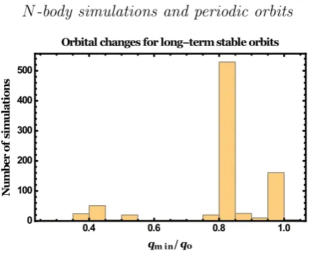
Figure 5. Number of stable systems integrated over 14 Gyr which experience a given maximum change in pericentre distance. Although this distribution is likely reflective of our initial condi-tion choices, the lowest value of about 0.4 is more importantly probably reflective of a global minimum.

unstable periodic orbits. The two main consequences of this finding are (1) the planar CRTBP 2:1 architecture cannot produce long-timescale (& 0.3% of the age of the universe) collisions, and (2) that this architecture cannot explain ob-served rates of WD pollution, in line with the findings of Frewen & Hansen (2014). We will discuss these points more in Section 5.

4.2 Orbital variations

For studies relevant to WD pollution, a particularly impor-tant orbital quantity to measure is how the pericentre dis-tanceq changes with time. Letq0 represent the initial peri-centre distance andqmin represent the minimum value ofq achieved throughout the simulation. We plotqmin/q0in Fig. 5 for all simulations which remained stable and ran for the age of the Universe.

This distribution is naturally highly-dependent on the initial conditions we chose for our simulations. The peak aroundqmin/q0≈0.8 might simply reflect this dependency. However, because we deliberately attempted to sample key

unstableregions of phase space, the minimum ratio attained

of qmin/q0 ≈ 0.4 is likely to be representative of a global minimum. At least, achieving a value less than about 0.4 is highly unlikely (at the 0.1% level). A value of 0.4 does not allow the asteroid to get remotely close to the Roche radius of the WD unless the initial pericentre is set to within about 0.02 au, which is only possible due to a scattering event after the parent star has become a WD.

4.3 Varying pairs ofaA and eA

(black). Hence, stability as defined in the N-body simula-tions does not reflect the long-term stability in the vicinity of stable periodic orbits where the motion is regular, but solely the absence of ejection, collision with the star, or col-lision with the planet. As we have already mentioned in Sec-tion 2.1, chaotic orbits are detected in the neighbourhood of unstable periodic orbits. In some cases, despite the irregu-larity in the evolution, the initial orbital elements do not change significantly over time and thus, these orbits can be considered as “stable” (see e.g. the examples in Section 4.5). Hence, our comparisons are inexact: Fig. 1 displays the periodic orbits as well as the DFLI maps, whereas Fig. 6 strictly illustrates qualitative system outcomes. In this figure we observe

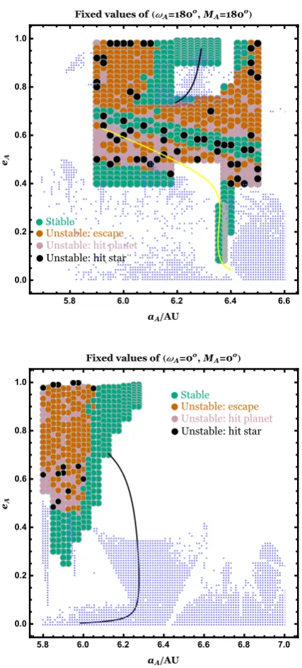
(i) Distinct blocks of stable systems. The locations of sev-eral of these blocks correspond to both regions which are close to stable periodic orbits and to regions containing DFLI regular orbits. One diagonal strip of stable systems, however, on the upper panel of Fig. 6 with 0.5≤eA≤0.7, is not a solid block, but instead is punctuated with collisional instability. A solid stable block also encompasses the lower tail (eA & 0.4) of the unstable periodic orbit family (the gray dots represent densely-packed green dots). In this tail, the DLFI includes a mixture of regular and chaotic orbits and does not tend strongly towards either type.

(ii) Distinct blocks of unstable systems. These blocks do encompass DFLI chaotic orbit regions. One unstable block surrounds the upper portion (eA&0.4) of the unstable pe-riodic orbit family. This block features a mix of all types of instability.

(iii) An inhomogeneous distribution of incidents of star-asteroid and star-planet collisions throughout the phase space. Escape is the dominant form of instability in these systems, and appear in blocks. For the WD case, all colli-sions occur on too short of a timescale (under 36 Myr) to explain Gyr pollution timescales, regardless of the collision distribution in phase space.

Overall, the correspondence between periodic orbits, DLFI maps, and long-term N-body simulations is robust. The low-eccentricity tail of the family of unstable periodic orbits is the most intriguing discrepancy, at first glance. Poincar´e surface of sections have on the one hand, revealed that the chaotic regions are bounded and hence, escape can-not occur. On the other hand, they showed that such regions are sensitive to Jupiter’s eccentricity (see e.g. Michtchenko & Ferraz-Mello 1995; Nesvorn´y & Ferraz-Mello 1997; Had-jidemetriou & Voyatzis 2000). Furthermore, the results of N-body simulations shown in Fig. 6 and depicting the ex-istence of islands of stability within chaotic regions as aA and eA vary in each configuration (i.e. when ωA = 0◦ or

ωA= 180◦) are in good agreement with the results presented with surfaces of section in Morbidelli & Moons (1993).

4.4 Varying pairs ofMA and ωA

Now let us explore this correspondence with the DFLI maps on plane (MA, ωA) from Fig. 3. These phase portraits illus-trate how stability changes asMAandωAare varied, instead of aA and eA. These portraits do intersect with both un-stable and un-stable periodic orbits at the points given in that

Figure 6. Stability portrait from 14 GyrN-body simulations for fixed (ωA, MA). Green spheres indicate stable systems and other

dots indicate unstable systems. Red, brown and black spheres re-spectively refer to systems where the asteroid escaped, hit the planet, and hit the star. The gray-looking spheres are the result of densely packed green spheres. These plots should be compared with Fig. 1; Families of stable (black) and unstable (yellow) pe-riodic orbits, as well as grid points wherelog(DF LI)≤1.2 (pale blue triangular symbols) are overplotted.

figure caption, but essentially focus on the regions surround-ing those orbits. The regions of greatest interest to us are the yellow strips, which are filled with irregular orbits that

maybecome unstable on the timescales we are interested in (Gyr).

3. For each point in each plot in Fig. 7, we ran multiple sim-ulations at different values ofeA(provided in the caption). We observe

(i) Variations ineAon the order of hundredths often com-pletely changes the outcome of the simulations. In the top plot, at a given point, as eA increases, unstable systems give way to stable systems, because the island of stability is reached (compare Figs. 1a, 3a and 4). These unstable sys-tems predominately feature escape. In the middle plot, at a given point, as eA increases, stable systems give way to unstable systems (which are a mix of escape and collisions), because the chaotic region for the semimajor axis that is fixed begins roughly when eA >0.4 (compare Figs. 1a, 3b and 4). In the bottom plot, nearly all the simulations become unstable. However, the character of the instability changes as one varieseA. At no point in any of the three plots are all concentric circles the same colour.

(ii) For a fixed value ofeA, as one moves along the strips, the outcome of the simulations (stable or unstable) remains largely the same. This trend is apparent in all three plots.

(iii) Collisions between the asteroid and star are inhomo-geneously and infrequently distributed. In no set of concen-tric circles are more than two coloured black.

(iv) The two (they are equivalent) exceptions in the bot-tom plot feature green concentric circles of nearly all stable simulations. They are linked with the outcome that is also seen in the top panel of Fig. 6 for this specific range in the eccentricities and the fixed value of the semimajor axis and justified therein accordingly (compare Figs. 1a, 3c and 4). Also, note how the frequency of green circles decreases as one strays from these equivalent configurations.

Overall, Figs. 3 and 7 demonstrate the importance of the initial orbital angles of the asteroid when determining long-term stability. The role of eccentricity is crucial, and demonstrates predictive power with clear trends.

4.5 Specific evolution examples

Even within the confines of the 2:1 planar CRTBP, the aster-oid’s osculating orbit may remain nearly static or vary dra-matically depending on its initial conditions. Consequently, there is no one representative orbit. Nevertheless, in this subsection we provide a few examples of asteroid evolution in order to at least impart to the reader a flavour of the variety seen across the simulations.

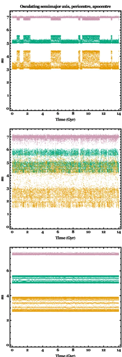
First consider Fig. 8, which exhibits the evolution for three simulations with identical initial orbital parameters (given in the caption) except for eA. AseA increases from 0.35 to 0.458 across the three simulations, the qualitative behaviour of the osculating orbit changes in unpredictable ways. The pericentre variation is greatest for the middle panel (from about 1.5 au to 6.0 au). In the top panel, the or-bit oscillates back and forth between two different modes of evolution. In the bottom panel, the semimajor axis and peri-centre appear to be rigidly bound within differently-sized ranges. When evaluating these plots, please recall that the output resolution for our simulations was 1 Myr.

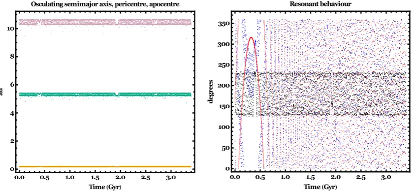
Figure 9 illustrates a more extreme case, where the as-teroid is initially highly eccentric (eA= 0.97). For this sys-tem, we show the evolution of the two 2:1 MMR angles in the right panel (black and blue), along with the evolution of

Figure 7. Stability portrait from 14 Gyr N-body simu-lations for fixed aA. Dots of different sizes refer to fixed

values of eA. The largest to smallest dots refer to (top panel) eA = {0.86,0.88,0.90,0.95,0.97,0.99}, (middle panel)

the apsidal angle (red). The black dots clearly librate about 180◦with an amplitude of nearly 50◦. The semimajor axis, pericentre and apocentre appear to change little, although the stray purple and green dots below the main stripes in-dicate brief but potentially dramatic swings from the initial orbit. Inhomogeneities in the stripes themselves (at about 0.4 Gyr and 1.9 Gyr) show up in the right panel as very slow oscillations in the black curves. Alternatively, the dra-matically slow circulatory motion indicated by the blue and red curves at about 0.3 Gyr does not appear to manifest itself in the left panel. In order to test if these features are a result of aliasing, we have run 5 additional simulations, each for 7 Gyr. In these simulations, the original output intervals were decreased by factors of 10, 7, 5, 3 and 2. The results demonstrate that the resonance in Fig. 9 appears to be real. In all cases, the angle librates and never deviates from the above-mentioned range.

5 DISCUSSION

In order to place our findings in the proper context, we con-sider here how they relate to real planetary systems. Partly due to history and to the voluminous and accurate set of available Solar system asteroid data, the vast majority of literature on long-term asteroid evolution is Solar System-specific (e.g. Bottke et al. 2000; Morbidelli 2002b; O’Brien & Sykes 2011). Inherent in Solar system studies are assump-tions about orbital architectures and radiative physics which do not necessarily apply in extrasolar systems, especially post-main-sequence exosystems.

5.1 Comparison with Solar system studies

The Solar system is different from the planar CRTBP be-cause the former contains more than one planet, and all of the Solar system planets have eccentric orbits which are at least slightly noncoplanar with asteroids and the Sun. Con-sequently, collisions with the Sun can occur through scat-tering interactions with multiple planets, leading to a much higher fraction of collisions than in our case (Farinella et al. 1994; Gladman et al. 1997; Minton & Malhotra 2010). The presence of multiple planets does not, however, preclude the possibility of long-lived (on Gyr timescale) stable “islands” where asteroids can reside in or close to the 2:1 mean mo-tion resonance with Jupiter (Chrenko et al. 2015). Asteroids in such islands may also be shaped by radiation-based per-turbations such as the Yarkovsky effect (Broˇz et al. 2005), which can affect the long-term evolution (Broˇz & Vokrouh-lick´y 2008) in ways that are missed in the the planar CRTBP studied herein.

5.2 Comparison with WD system studies

In contrast, extrasolar systems offer a wide variety of archi-tectures, The majority of all known exosystems contain one exoplanet, leaving open the possibility of the RTBP being widely applicable outside of our Solar system. Individual as-teroids are currently undetectable, except in WD systems, where their tidally-shorn innards are observed orbiting WDs or accreting onto them.

Asteroids, comets and planets which orbit stars that

Figure 8. The evolution of the semimajor axis (green), pericen-tre (yellow) and apocenpericen-tre (purple) of an asteroid in three indi-vidual systems. In all three systems,aA= 5.95 au,ωA= 0.0◦and

MA= 0.0◦. In the top, middle and bottom panels, respectively,

eA={0.35,0.4148,0.458}. The plots illustrate different

Figure 9. The evolution of an initially and otherwise highly eccentric system (eA= 0.97) system which exhibits some resonant behaviour.

Other initial parameters areaA= 6.2517 au,ωA= 195◦andMA= 100◦. The left panel illustrates the evolution of the semimajor axis

(green), pericentre (orange) and apocentre (purple), and the right panel illustrates the evolution of the two resonant 2:1 angles (black and blue) and the apsidal angle (red). The black points, which correspond to the resonant angle which includes the asteroid’s argument of pericentre, appears to librate about 180◦throughout the 3.5 Gyr of evolution shown, and shows two distinctive features at about 0.4 Gyr and 1.9 Gyr. The circulating apsidal angle is slowest at about 0.3 Gyr.

leave the main sequence become subject to an assortment of important physical processes whose previous influence was negligible:

(i) Stellar mass loss, which causes an outward expansion and possible stretching and breaking of a bound osculat-ing orbit (Omarov 1962; Hadjidemetriou 1963; Veras et al. 2011a; Adams et al. 2013; Veras et al. 2013a; Voyatzis et al. 2013)

(ii) Stellar radius enlargement, leading to engulfment or tidal disruption (Villaver & Livio 2009; Kunitomo et al. 2011; Mustill & Villaver 2012; Adams & Bloch 2013; Nord-haus & Spiegel 2013; Villaver et al. 2014; Staff et al. 2016), (iii) Stellar wind drag, which usually acts in opposition to mass loss (Bonsor & Wyatt 2010; Dong et al. 2010; Veras et al. 2015a)

(iv) Variations in stellar luminosity, which lead to YORP-induced fission (Veras et al. 2014a), Yarkovsky-YORP-induced dis-persion (Veras et al. 2015a), inward drag from radiation pres-sure and Poynting-Robertson effects (Bonsor & Wyatt 2010; Dong et al. 2010; Veras et al. 2015b) and sublimation (Veras et al. 2015c)

These effects redistribute surviving bodies and debris in complex and still poorly-understood ways. Regardless, ob-servations reveal that this material somehow is frequently and significantly perturbed close to, and ultimately onto, the resulting WD. In fact planetary remnants are directly detected in the atmospheres of between one quarter and one half of all Milky Way WDs (Zuckerman et al. 2003, 2010; Koester et al. 2014). These signatures are referred to as

pol-lution and are thought to arise from accretion from

com-pact discs (Rafikov 2011a,b; Metzger et al. 2012; Rafikov & Garmilla 2012; Wyatt et al. 2014) which are readily observed (e.g. Bergfors et al. 2014; Rocchetto et al. 2014; Wilson et al. 2014; Raddi et al. 2015) and are thought to have formed by the tidal disruption of incoming planetary bodies (Graham

et al. 1990; Jura 2003; Debes et al. 2012; Bear & Soker 2013; Veras et al. 2014b), such as those disintegrating around WD 1145+017 (Vanderburg et al. 2015). WD pollution reveals the chemical composition of the accreeted bodies (Zucker-man et al. 2007; G¨ansicke et al. 2012; Farihi et al. 2013; Jura & Young 2014; Xu et al. 2014) and consequently provides unambiguous bulk density data about exoplanetary interi-ors.

Asteroids which pollute WDs must be on highly eccen-tric orbits because in order to avoid engulfment during the giant branch (GB) stages of stellar evolution, the semimajor axis must be at least a few au. In order to be perturbed into highly eccentric orbits, asteroids need instigators. Three in-vestigations (Bonsor et al. 2011; Debes et al. 2012; Frewen & Hansen 2014) have dynamically modelled the interaction of asteroids with one planet during the GB phases of evolution, as well as up to 1 Gyr during the WD phase. Bonsor & Ve-ras (2015) considered the consequences of a perturbation by a wide orbit stellar companion, and Payne et al. (2016a,b) determined how liberated moons would contribute to the dynamical architecture.

However, none of those studies included simulations which incorporated the Yarkovsky effect nor stellar wind drag (although see Section 5.1 of Frewen & Hansen 2014), which could represent the dominant drivers of asteroid evo-lution during the GB phase (Veras et al. 2015a). Therefore, how asteroids evolve during GB evolution, supposing they survive rotational spin-up (Veras et al. 2014a), remains an open question, one that we do not address here.

star-planet plane (J. Debes, private communication) in or-der to demonstrate their theory. Frewen & Hansen (2014) later explicitly explored how the eccentricity of the planet affects collision rates with the WD when the asteroid was confined to within 0.5◦of the WD-planet plane. They found thateP>0.02 is a necessary condition to pollute WDs with a sufficiently high amount of material to extrapolate to ob-servations.

Although the numerical simulations of both studies ran for up to only 1 Gyr, our results affirm theirs and strin-gently rule out dynamical pollution mechanisms with a sin-gle planet on a circular orbit at the 2:1 commensurability. The small inclinations adopted by Frewen & Hansen (2014) suggests that the driver for collisions is planetary eccentric-ity rather than non-coplanareccentric-ity. Regardless, undertaking a systematic study for each of these orbital parameters – as well as different commensurabilities – is now required in order to pinpoint the most likely physical origin of long-timescale collisions with the WD. Periodic orbits represent an effective tool for this purpose, especially since so many families have already been computed.

6 CONCLUSION

We have evaluated the predictive power of periodic orbits and their phase space surroundings to determine the long-term (1-14 Gyr) stability of systems containing one star, one planet and one asteroid in the planar CRTBP. We utilized the three families of periodic orbits which are associated with the 2:1 MMR, such that the asteroid is interior to the planet. Our resource-consuming 14 Gyr simulations revealed good agreement between the final dynamical outcome and the structure of phase space about the periodic orbits. Con-sequently, researchers can use these orbits as broadly reliable guides to choose sets of initial conditions (a(N)_A , eA, ωA, MA) forN-body simulations to predict whether a given system will remain stable over the age of the Universe.

Of particular interest for Gyr-old WDs which host cir-cumstellar debris discs and atmospheric metal pollution are

unstable planetary systems that feature very late collisions

between the asteroid and star. Therefore, in this paper we have focused on unstable cases. Despite this emphasis, in none of our simulations did a collision occur after 36 Myr, thereby providing analytical backing to the findings of Frewen & Hansen (2014) that a circular planet fails to pollute WDs with a sufficient number of asteroids at suffi-ciently late ages.

ACKNOWLEDGMENTS

We would like to thank the reviewer, A. Mustill, for his comments with regards to the figures, whose implementation enhanced our paper. We thank John H. Debes and Matthew J. Holman for useful discussions. DV benefited by support by the European Union through ERC grant number 320964.

REFERENCES

Adams, F. C., Anderson, K. R., & Bloch, A. M. 2013, MNRAS, 432, 438

Adams, F. C., & Bloch, A. M. 2013, ApJL, 777, LL30

Agol, E., Steffen, J., Sari, R., & Clarkson, W. 2005, MNRAS, 359, 567

Alcock, C., Fristrom, C. C., & Siegelman, R. 1986, ApJ, 302, 462 Alonso, R., Rappaport, S., Deeg, H. J., & Palle, E. 2016, A&A,

589, L6

ALMA Partnership, A., Brogan, C. L., Perez, L. M., et al. 2015, arXiv:1503.02649, ApJL In press.

Antoniadou, K. I., 2014, Dynamics of planetary systems in reso-nances: From the planar to the spatial case, PhD thesis, Aris-totle University of Thessaloniki, GR

Antoniadou, K. I., 2016, EPJ ST, 225, 1001.

Antoniadou, K. I., Voyatzis, G., & Kotoulas, T. 2011, IJBC, 21, 2211

Antoniadou, K. I., & Voyatzis, G. 2013, CeMDA, 115, 161 Antoniadou, K. I., & Voyatzis, G. 2014, Ap&SS, 349, 657 Antoniadou, K. I., & Voyatzis, G. 2016, MNRAS, 461, 3822 Antoniadou, K. I., Voyatzis, G., & Varvoglis, H. 2014, Proceedings

of IAU, 9, 82, doi:10.1017/S1743921314007893

Armstrong, D. J., Veras, D., Barros, S. C. C., et al. 2015, arXiv:1503.00692, Submitted to A&A

Beaug´e, C. 1994, CeMDA, 60, 225

Beaug´e, C., Ferraz-Mello, S., & Michtchenko, T. A. 2003, ApJ, 593, 1124

Bear, E., & Soker, N. 2013, New Astronomy, 19, 56

Bergfors, C., Farihi, J., Dufour, P., & Rocchetto, M. 2014, MN-RAS, 444, 2147

Bonsor, A., & Wyatt, M. 2010, MNRAS, 409, 1631 Bonsor, A., & Wyatt, M. 2012, MNRAS, 420, 2990

Bonsor, A., Mustill, A. J., & Wyatt, M. C. 2011, MNRAS, 414, 930

Bonsor, A., & Veras, D. 2015, MNRAS, 454, 53

Bottke, W. F., Jedicke, R., Morbidelli, A., Petit, J.-M., & Glad-man, B. 2000, Science, 288, 2190

Bozis, G., & Hadjidemetriou, J. D. 1976, Celestial Mechanics, 13, 127

Broˇz, M., Vokrouhlick´y, D., Roig, F., et al. 2005, MNRAS, 359, 1437

Broˇz, M., & Vokrouhlick´y, D. 2008, MNRAS, 390, 715 Chambers, J. E. 1999, MNRAS, 304, 793

Chrenko, O., Broˇz, M., Nesvorn´y, D., Tsiganis, K., & Skoulidou, D. K. 2015, MNRAS, In Press, arXiv:1505.04329

Croll, B., Dalba, P. A., Vanderburg, A., et al. 2015, arXiv:1510.06434

Davies, M. B., Adams, F. C., Armitage, Chambers, J., Ford, E., Morbidelli, A., Raymond, S. N., Veras, D. 2014, Protostars and Planets VI, 787

Debes, J. H., Walsh, K. J., & Stark, C. 2012, ApJ, 747, 148 Dong, R., Wang, Y., Lin, D. N. C., & Liu, X.-W. 2010, ApJ, 715,

1036

Duncan, M. J., & Lissauer, J. J. 1998, Icarus, 134, 303

Farihi, J., Dufour, P., Napiwotzki, R., & Koester, D. 2011, MN-RAS, 413, 2559

Farihi, J., G¨ansicke, B. T., & Koester, D. 2013, Science, 342, 218 Farihi, J. 2016, New Astronomy Reviews, 71, 9

Farinella, P., Froeschl´e, C., Froeschl´e, C., et al. 1994, Nature, 371, 314

Frewen, S. F. N., & Hansen, B. M. S. 2014, MNRAS, 439, 2442 Froeschl´e, C., Lega, E., & Gonczi, R. 1997, CeMDA, 67, 41 G¨ansicke, B. T., Koester, D., Farihi, J., et al. 2012, MNRAS, 424,

333

G¨ansicke, B. T., Aungwerojwit, A., Marsh, T. R., et al. 2016, ApJL, 818, L7

Gladman, B. J., Migliorini, F., Morbidelli, A., et al. 1997, Science, 277, 197

Graham, J. R., Matthews, K., Neugebauer, G., & Soifer, B. T. 1990, ApJ, 357, 216

Hadjidemetriou, J. D. 1975, Celestial Mechanics, 12, 155 Hadjidemetriou, J. D. 1984, Celestial Mechanics, 34, 379 Hadjidemetriou, J. D. 1993, CeMDA, 56, 201

Hadjidemetriou, J. D. 2006, CeMDA, 95, 225

Hadjidemetriou J., Voyatzis G., 2000, CeMDA, 78, 137

Haghighipour, N., Couetdic, J., Varadi, F., & Moore, W. B. 2003, ApJ, 596, 1332

H´enon, M. 1997, Generating Families in the Restricted Three-Body Problem, Springer

Hinse, T. C., Christou, A. A., Alvarellos, J. L. A., & Go´zdziewski, K. 2010, MNRAS, 404, 837

Holman, M. J., & Murray, N. W. 1996, AJ, 112, 1278 Jura, M. 2003, ApJL, 584, L91

Jura, M., Xu, S., Klein, B., Koester, D., & Zuckerman, B. 2012, ApJ, 750, 69

Jura, M., & Young, E. D. 2014, Annual Review of Earth and Planetary Sciences, 42, 45

Klein, B., Jura, M., Koester, D., Zuckerman, B., & Melis, C. 2010, ApJ, 709, 950

Klein, B., Jura, M., Koester, D., & Zuckerman, B. 2011, ApJ, 741, 64

Laughlin, G., Chambers, J., & Fischer, D. 2011, ApJ, 579, 455 Koester, D., Girven, J., G¨ansicke, B. T., & Dufour, P. 2011, A&A,

530, AA114

Koester, D., G¨ansicke, B. T., & Farihi, J. 2014, A&A, 566, AA34 Kunitomo, M., Ikoma, M., Sato, B., Katsuta, Y., & Ida, S. 2011,

ApJ, 737, 66

Lee, M. H., & Thommes, E. W. 2009, ApJ, 702, 1662

Libert, A.-S., & Sansottera, M. 2013, Celestial Mechanics and Dynamical Astronomy, 117, 149

Manser, C., et al. 2015, In Prep

Marchal, C. 1990, The three-body problem, Elsevier

Metzger, B. D., Rafikov, R. R., & Bochkarev, K. V. 2012, MN-RAS, 423, 505

Michtchenko, T. A., Beaug´e, C., & Ferraz-Mello, S. 2006, CeMDA, 94, 411

Michtchenko, T. A., Beaug´e, C., & Ferraz-Mello, S. 2008, MN-RAS, 387, 747

Michtchenko T. A., Ferraz-Mello S. 1995, A&A, 303, 945 Minton, D. A., & Malhotra, R. 2010, Icarus, 207, 744

Morbidelli, A. 2002a, Modern celestial mechanics : aspects of solar system dynamics, by Alessandro Morbidelli. London: Taylor & Francis, 2002, ISBN 0415279399

Morbidelli, A. 2002b, Annual Review of Earth and Planetary Sci-ences, 30, 89

Morbidelli, A., & Moons, M. 1993, Icarus, 102, 316

Murray, C. D., & Dermott, S. F. 1999, Solar system dynamics Murray, N., & Holman, M. 1997, AJ, 114, 1246

Mustill, A. J., & Villaver, E. 2012, ApJ, 761, 121

Mustill, A. J., Veras, D., & Villaver, E. 2014, MNRAS, 437, 1404 Naoz, S. 2016, ARA&A In Press, arXiv:1601.07175

Nesvorn´y, D. & Ferraz-Mello, S. 1997, A&A, 320, 672 Nesvorn´y, D., Kipping, D., Terrell, D., et al. 2013, ApJ, 777, 3 Namouni, F., & Morais, M. H. M. 2015, MNRAS, 446, 1998 Naoz, S., Farr, W. M., Lithwick, Y., Rasio, F. A., & Teyssandier,

J. 2013, MNRAS, 431, 2155

Nordhaus, J., & Spiegel, D. S. 2013, MNRAS, 432, 500

O’Brien, D. P., & Sykes, M. V. 2011, Solar System Reviews, 163, 41

Omarov, T. B. 1962, Izv. Astrofiz. Inst. Acad. Nauk. KazSSR, 14, 66

Payne, M. J., Veras, D., Holman, M. J., G¨ansicke, B. T. 2016a, MNRAS, 457, 217

Payne, M. J., Veras, D., G¨ansicke, B. T., Holman, M. J. 2016b, Submitted to MNRAS

Raddi, R., G¨ansicke, B. T., Koester, D., et al. 2015, Submitted to MNRAS

Rafikov, R. R. 2011a, MNRAS, 416, L55

Rafikov, R. R. 2011b, ApJL, 732, LL3

Rafikov, R. R., & Garmilla, J. A. 2012, ApJ, 760, 123

Rappaport, S., Gary, B. L., Kaye, T., et al. 2016, MNRAS, 458, 3904

Rocchetto, M., Farihi, J., Gaensicke, B. T., & Bergfors, C. 2014, arXiv:1410.6527

Schr¨oder, K.-P., & Connon Smith, R. 2008, MNRAS, 386, 155 Staff, J. E., De Marco, O., Wood, P., Galaviz, P., & Passy, J.-C.

2016, MNRAS, 458, 832

Stone, N., Metzger, B. D., & Loeb, A. 2015, MNRAS, 448, 188 Thommes, E. W., & Lissauer, J. J. 2010, ApJ, 597, 566 Tsiganis, K., Varvoglis, H., & Hadjidemetriou, J. D. 2002, Icarus,

159, 284

Vanderburg, A., Johnson, J. A., Rappaport, S., et al. 2015, Na-ture, 526, 546

Varadi, F. 1999, AJ, 118, 2526

Veras, D. 2007, Celestial Mechanics and Dynamical Astronomy, 99, 197

Veras, D., & Armitage, P. J. 2007, ApJ, 661, 1311 Veras, D., & Ford, E. B. 2010, ApJ, 715, 803

Veras, D., Wyatt, M. C., Mustill, A. J., Bonsor, A., & Eldridge, J. J. 2011a, MNRAS, 417, 2104

Veras, D., Ford, E. B., & Payne, M. J. 2011b, ApJ, 727, 74 Veras, D., & Ford, E. B. 2012, MNRAS, 420, L23

Veras, D., & Wyatt, M. C. 2012, MNRAS, 421, 2969

Veras, D., Hadjidemetriou, J. D., & Tout, C. A. 2013a, MNRAS, 435, 2416

Veras, D., Mustill, A. J., Bonsor, A., & Wyatt, M. C. 2013b, MNRAS, 431, 1686

Veras, D., & Mustill, A. J. 2013, MNRAS, 434, L11 Veras, D., & Evans, N. W. 2013, MNRAS, 430, 403

Veras, D., Jacobson, S. A., G¨ansicke, B. T. 2014a, MNRAS, 445, 2794

Veras, D., Leinhardt, Z. M., Bonsor, A., & G¨ansicke, B. T. 2014b, MNRAS, 445, 2244

Veras, D., Shannon, A., G¨ansicke, B. T. 2014c, MNRAS, 445, 4175

Veras, D., Eggl, S., & G¨ansicke, B. T. 2015a, In Press, arXiv:1505.01851

Veras, D., Leinhardt, Z.M., Eggl, S., & G¨ansicke, B. T. 2015b, In Press, MNRAS, arXiv:1505.06204

Veras, D., Eggl, S., & G¨ansicke, B. T. 2015c, In Press, MNRAS, arXiv:1506.07174

Veras, D., G¨ansicke, B. T. 2015, MNRAS, 447, 1049 Veras, D. 2016, Royal Society Open Science, 3, 150571

Veras, D., Mustill, A. J., G¨ansicke, B. T., et al. 2016, MNRAS, 458, 3942

Villaver, E., & Livio, M. 2009, ApJL, 705, L81

Villaver, E., Livio, M., Mustill, A. J., & Siess, L. 2014, ApJ, 794, 3

Voyatzis, G. 2008, ApJ, 675, 802

Voyatzis, G., Antoniadou, K. I., & Tsiganis, K. 2014, CeMDA 119, 221

Voyatzis, G., & Hadjidemetriou, J. D. 2005, CeMDA, 93, 263 Voyatzis, G., Hadjidemetriou, J. D., Veras, D., & Varvoglis, H.

2013, MNRAS, 430, 3383

Voyatzis, G., Kotoulas, T., & Hadjidemetriou, J. D. 2005, CeMDA, 91, 191

Voyatzis, G., Kotoulas, T., & Hadjidemetriou, J. D. 2009, MN-RAS, 395, 2147

Wilson, D. J., G¨ansicke, B. T., Koester, D., et al. 2014, MNRAS, 445, 1878

Wilson, D. J., G¨ansicke, B. T., Koester, D., et al. 2015, MNRAS, 451, 3237

Wilson, D. J., G¨ansicke, B. T., Farihi, J., & Koester, D. 2016, MNRAS In Press, arXiv:1604.03104

Xu, S., Jura, M., Klein, B., Koester, D., & Zuckerman, B. 2013, ApJ, 766, 132

Xu, S., Jura, M., Koester, D., Klein, B., & Zuckerman, B. 2014, ApJ, 783, 79

Xu, S., & Jura, M. 2014, ApJL, 792, L39

Xu, S., Jura, M., Dufour, P., & Zuckerman, B. 2016, ApJL, 816, L22

Zhou, G., Kedziora-Chudczer, L., Bailey, J., et al. 2016, arXiv:1604.07405

Zuckerman, B., Koester, D., Reid, I. N., H¨unsch, M. 2003, ApJ, 596, 477

Zuckerman, B., Koester, D., Melis, C., Hansen, B. M., & Jura, M. 2007, ApJ, 671, 872

Zuckerman, B., Melis, C., Klein, B., Koester, D., & Jura, M. 2010, ApJ, 722, 725

This paper has been typeset from a TEX/LA_{TEX file prepared by}