Multi coil focused EMAT for characterisation of surface breaking defects of arbitrary orientation

Original citation:

Thring, C. B., Fan, Yichao and Edwards, R. S. (Rachel S.). (2017) Multi-coil focused EMAT for

characterisation of surface-breaking defects of arbitrary orientation. NDT & E International,

88. pp. 1-7

Permanent WRAP URL:

http://wrap.warwick.ac.uk/89546

Copyright and reuse:

The Warwick Research Archive Portal (WRAP) makes this work by researchers of the

University of Warwick available open access under the following conditions. Copyright ©

and all moral rights to the version of the paper presented here belong to the individual

author(s) and/or other copyright owners. To the extent reasonable and practicable the

material made available in WRAP has been checked for eligibility before being made

available.

Copies of full items can be used for personal research or study, educational, or not-for-profit

purposes without prior permission or charge. Provided that the authors, title and full

bibliographic details are credited, a hyperlink and/or URL is given for the original metadata

page and the content is not changed in any way.

Publisher’s statement:

© 2017, Elsevier. Licensed under the Creative Commons

Attribution-NonCommercial-NoDerivatives 4.0 International

http://creativecommons.org/licenses/by-nc-nd/4.0/

A note on versions:

The version presented here may differ from the published version or, version of record, if

you wish to cite this item you are advised to consult the publisher’s version. Please see the

‘permanent WRAP URL’ above for details on accessing the published version and note that

access may require a subscription.

Multi-coil focused EMAT for characterisation of

surface-breaking defects of arbitrary orientation

C.B. Thring, Y. Fan, R.S. Edwards

Department of Physics, University of Warwick, Coventry CV4 7AL, United Kingdom

Abstract

Electromagnetic Acoustic Transducers (EMATs) are a useful ultrasonic tool for non-destructive evaluation in harsh environments due to their non-contact capabilities, and their ability to operate through certain coatings. This work presents a new Rayleigh wave EMAT transducer design, employing geometric focusing to improve the signal strength and detection precision of surface break-ing defects. The design is robust and versatile, and can be used at frequencies centered around 1 MHz. Two coils are used in transmission mode, which allows the usage of frequency-based measurement of the defect depth. Using a 2 MHz driving signal, a focused beam spot with a width of 1.3±0.25 mm and a focal depth of 3.7 ±0.25 mm is measured, allowing for defect length measurements with an accuracy of±0.4 mm and detection of defects as small as 0.5 mm depth and 1 mm length. A set of four coils held under one magnet are used to find defects at orientations offset from normal to the ultrasound beam propagation direction. This EMAT has a range which allows detection of defects which prop-agate at angles from 16◦ to 170◦ relative to the propagation direction over the range of 0 to 180◦, and the set up has the potential to be able to detect defects propagating at all angles relative to the wave propagation direction if two coils are alternately employed as generation coils.

Keywords: Ultrasonics, EMAT, Focusing, Rayleigh wave, Surface-breaking defects

1. Introduction

Ultrasonic surface waves, and in particular Rayleigh waves, have been shown to be an effective tool for the detection of surface breaking defects, includ-ing rollinclud-ing contact fatigue (RCF) [1] and stress corrosion crackinclud-ing (SCC) [2]. Rayleigh waves are generally used in one of two modes of operation; looking for reflections returned by surface breaking defects [3], or measuring varia-tions in the transmitted signal traveling from a generation to a detection

ducer [4, 5]. Any variation in the received signal indicates there has been inter-action with a defect incident in the beam path, or a change in the generation or detection conditions. In addition, when a transducer is scanned directly over a surface-breaking defect, signal enhancement occurs due to interference of the incident and reflected wavemodes [6, 7, 8], giving a useful factor for identifying the position.

The majority of the Rayleigh wave energy travels within one wavelength of the sample surface [9], and as such the interaction between a Rayleigh wave and a defect is highly dependent on the wavelength and the defect depth; a defect of comparable depth to the wavelength will block most of the signal from being transmitted, while a shallower one will have less of an effect [10]. The use of a broadband wave, as typically generated by an electromagnetic acoustic transducer (EMAT), enables analysis of the frequencies which are transmitted and hence a measure of defect depth [4].

EMATs are a non-contact technique for generating and detecting ultrasound, and are especially suited to harsh environments [11, 12]. The main component is a coil of wire, typically flat and parallel to the surface under inspection. A strong AC pulse is transmitted through the coil, generating a corresponding alternating magnetic field. If there is an electrically conducting sample nearby, the fluctuating magnetic field generates a mirror current within the sample. The interaction of this with the dynamic magnetic field and any external static magnetic field via the Lorentz force leads to ultrasound generation [11, 13]. Detection works similarly in reverse, except that the magnet becomes essential, and the efficiency is greatly improved as it is detecting moving electrons rather than using electron motion to excite the sample bulk [13, 14]. As the mechanism works via electromagnetic induction the transducer does not need to be in direct contact with the sample and no couplant is required, offering the potential for fast scanning and easy use on rough, hot and rusted surfaces, and through certain coatings.

For early stage detection of surface breaking defects, sub-millimeter defect detection is needed [15]. Several techniques are available, with the main one being eddy current testing. However, in some industries a partially conducting paint coating is used to protect the component under test. Standard eddy current testing is then not suitable as frequencies above about 300 kHz generate purely within the coating due to the skin depth. An alternative technique is to use EMATs which can operate through such coatings, and can be designed to operate at high temperatures.

shaping of the coil to create a shear wave beam spot on the opposite surface of the sample to the probe [19], and a focused surface-wave meander line de-sign has been investigated for operation in reflection mode [20, 3]. Geometric focusing means that on, interacting with a defect not at the focal point, wave components are in fact incident at oblique angles, potentially complicating the interaction. However, the designs are intended for 2D surface scanning with the region of interest being the focal point. At this position the compound wave packet formed from waves from all parts of the shaped wavefront, using a Huygens approach, is approximately equivalent to an incident wave travelling at right angles to the defect due to interference of waves.

To ensure detection of defects with sub-millimetre depths, high frequencies are required; the EMAT reported in reference [3] was produced for operation at 2 MHz, but this requires a highly complex design. The transducer was very effective at detecting and sizing the surface-breaking profile of machined slot defects down to 1 mm in length. However, the complex design makes it less robust than standard EMATs, and the close proximity of having two large coils under one magnet creates a long dead-time (period of ringing due to the generation pulse) which increases with transducer lift-off, limiting its capabilities.

This work investigates a simplified, focused racetrack design, used in trans-mission but with all the coils held under a single magnet to allow for precise focal point alignment and scanning simplicity. The transmission technique and chosen coil extent allows the coils to be set far enough apart to decrease the dead-time, giving them the potential to perform at higher lift-off. Preliminary work on the design has been presented in a conference paper [21]. The use of a racetrack coil rather than a meander-line means the EMAT is not frequency tuned, and has a fairly broad band signal. The defect depth dependence of the transmitted frequencies was used to calibrate defect depths [4]. A set of four focused racetrack coils were then produced, all aligned around the same focal point. These can be used as one generator and three detectors, measur-ing transmission, reflection, and diffraction from defects at arbitrary angles to the wave propagation direction, giving the ability to pick up defects regardless of the orientation.This paper presents these results, alongside analysis of the transducer design and beam profile.

2. Transducer Design and Analysis

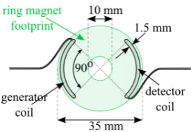
Figure 1: EMAT schematic showing racetrack pair. The magnetic field is orientated into the plane of the paper.

The central hole in the magnet gives several benefits. Foremost, it prevents the transmission of Rayleigh waves through the magnet and interfering with measurement of the arrival within the sample. Secondly, it removes any poten-tial contact of the transducer with the sample at the focal point, removing any loading at this position. Finally, it allows direct visual access to the sample surface facilitating accuracy in focal point positioning, and also permitting the characterisation of the focal point using a laser vibrometer.

The focal point characterisation was performed with the EMAT driving pulse produced by an adapted Ritec RAM-5000 pulser-receiver generating a 2 MHz, three cycle sinusoid output. The EMAT was placed on an aluminium sample and the surface visible through the ring magnet central hole was scanned using a laser vibrometer. Figure 2 (a) shows a snapshot at a time of 5.4µs after pulse generation, when the beam is at the focal point. The signal detected around the periphery is where the laser is incident on the magnet surface which is 20 mm higher than the sample surface on which the signal is being detected in the centre. This height change causes the laser beam to be out of focus, causing a strong increase in noise levels.

The signal power (figure 2(b)) was found by cross-correlating the raw data with a simulated generation signal designed to match the generated signal. The absolute value was then found, and the power obtained by squaring the result and finding the maximum signal peak after the generation noise. Full details are given in reference [3]. The simulated signal,G, was calculated over the same time range,t, as the real data using

G=e−(t−t0 )

2

2a2 _e2iπf(t−t0) ₍₁₎

where f is the frequency, t0 is the time offset, and a is the bandwidth of the

signal in the time domain. The values used to match the generation werea=1µs,

f=2 MHz, andt0=20µs.

The EMAT was found to focus to a 1.3 ± 0.25 mm width beam with a 3.7 ±0.25 mm focal depth. The aperture angle of the generation coil is 45◦, and hence any aperture effect is minimal; a smaller aperture angle will lead to changes in the focal beam profile [3].

Figure 3: Example detected EMAT signals in aluminium for a three cycle sinusoidal output, using 16 averages.

possible to generate [22]. However, narrowing the coil decreases the number of turns of wire, and thus weakens the overall signal. The Ritec driving signal was varied over the frequency range 0.5-3 MHz in 0.25 MHz increments, for both one and three cycles of a sinusoid output, and the corresponding signal generated in an aluminium sample was analysed to look for optimal operating conditions, using the second coil as a detector. Some example detected signals are shown in figure 3. An offset of 0.2 V has been used between each signal so that the signals can be easily compared. The signal wave packet in figure 3 clearly starts distorting above about 2 MHz. This indicates that the coil spatial extent is too wide for the high frequency wave to be efficiently generated [22].

The peak to peak signal as a function of driving frequency is shown in fig-ure 4 for both cycle settings. A 1 MHz driving frequency gives the strongest peak to peak signal for both cycle lengths. This is as expected, given the width of the coil, when approximating it as a linear coil [22]. The racetrack coil design has a more complicated dependence of frequency on width, but the linear ap-proximation gives a reasonable prediction of frequency behaviour. Decreasing the coils’ width to increase this frequency would decrease the signal strength due to the smaller footprint on the sample. For frequency depth gauging, a significant transmitted signal is necessary to characterise the depth [4], there-fore a broadband signal could be beneficial as there will be a wider range of frequencies to be transmitted under the defect. A one-cycle driving frequency gives a more broadband pulse, as expected. However, for very shallow defects the one-cycle generation may not contain sufficient high frequency content to detect them accurately and therefore three cycle generation is optimal.

3. Defect Length Measurement

Figure 4: Variation in detected EMAT signal strength in aluminium as a function of the frequency of the driving signal, for 1 and 3 cycle operation using 16 averages.

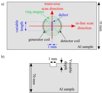
Figure 5: (a) EMAT scan set up for defect characterisation. (b) Defect cross section.

sub-millimetre defects, while still having a reasonably strong and undistorted signal. The defect profiles and scanning directions are shown in figure 5. Defects were artificially produced using a 1 mm diameter drill, giving rounded ends and a constant opening of 1 mm. The lengths were varied as 1, 3, 5, 7, 8, and 11 mm, and the depths were varied as 0.5, 1, 1.5, and 2 mm, giving a total of 24 simulated defects. The lengths include the 1 mm diameter curved edge; the 1 mm length defects are hence cylindrical drilled holes. A set of scans were performed, with two scan directions used; transverse and in-line, labeled in figure 5(a). Both scans were performed with the transducer orientation as depicted, and all data here-on is presented as single shot (no averaging) unless noted.

Figure 6: In-line scans of three different length, 2 mm depth defects. Lengths indicated in the headers. Each scan has been individually normalised to its own maximum.

is of sufficient size and in the correct position no signal will be transmitted. This effect is shown clearly in the figure; for the 1 mm length (cylindrical) defect even at the focal point there is still some transmission as the defect is smaller than the beam width, nevertheless, the defect is still detected. For the longer defects, a region of minimum signal power is found with the length of this region dependent on the length of the defect relative to the focal beam area. In a 1D scan, the effect of misalignment of coils relative to the defect recorded depends on defect length. For very small defects the depth may be underestimated. Deep defects wider than the transducer will block all signal once they are between the coils, and the effect of misalignment is negligible.

When the generator or detector coils pass over the defect, signal enhance-ment can be seen by the interference pattern and enhanceenhance-ment of signal power close to the defect (e.g. between 10-15 mm on the scan of the 3 mm length defect, figure 6). This effect has been studied in several works [7, 8]; the en-hancement is due to interference between the incident Rayleigh wave and the reflected and mode-converted waves from the defect. For the 5 mm length defect the enhancement is much stronger than for the shorter lengths, showing that it is reflecting the majority of the incident waves. The maximum signal within the expected Rayleigh wave arrival time was measured at each scan position and is shown in figure 7, with the focal beam at the centre of each defect set as a scan position of 0 mm. This shows the enhancement, with sharp signal spikes around±15 mm from the central position when the coils are incident over the defect, and the gradual blocking of the signal in the center.

Figure 7: Maximum signals from the in-line scans of three different length, 2 mm depth defects, from the data in figure 6. Lengths indicated in the legend.

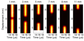
Figure 8: Transverse scans of six different length (indicated in the headers) 0.5 mm depth defects. Scans are individually normalised. The 5 mm length scan had a shorted scan length and the white segment at the end of the scan represents the area where no data was taken.

y-axes to indicate the change in scan direction. Again, the data has been cross-correlated and individually normalised to the maximum signal in each plot, and all defects are detected. Figure 9 shows the maximum signal power measured in the Rayleigh wave arrival time window at each position, normalised to the max-imum signal for all scans. Vertical dotted lines show the actual defect lengths. As can be seen, the defects block almost all of the signal at the center, except for the 1 mm diameter defect which still allows some noticeable transmission, as it is narrower than the beam width. There is still transmission beneath these shallow defects, as would be expected from the ultrasound wavelength, however the use of the cross-correlation technique gives a strong preference in the images produced to stronger signals, making it difficult to spot this transmission.

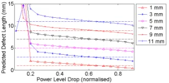
Figure 10: Predicted defect lengths depending on the signal level drop defined as sufficient to indicate the presence of a defect.

A drop in normalised signal power of 0.5 corresponds to a 3 dB drop, the usual threshold for ultrasonic signal detection. However, as the defects have rounded ends and the beam does not have a point-like focus, a 3 dB signal drop (or half power point) is not necessarily the best for measuring defect lengths. To analyse the data, the power level drop is defined as one minus the maximum signal, allowing a measurement of how much the signal power needs to drop by in order for the defect to be measured. The edges of the defects are defined as occurring when the power level drop reaches a chosen threshold. From figure 9 it is clear that requiring a large drop in signal power before a defect is indicated will give an underestimate of the length, whereas using a very small drop will lead to a noisy measurement and higher rate of false calls. Figure 10 shows the predicted defect length as a function of power level drop, with the actual defect lengths shown as dashed lines.

To compare data from all the different defects scanned, the power level drops at which the predicted lengths match the actual lengths have been interpolated from the data and are shown in figure 11. The 0.5 mm depth defects have a consistently lower optimum power level drop; for these shallow defects, some signal is always transmitted, giving reduced power level drops compared to the deeper defects. However, the figure indicates that a 0.7 power level drop would give reasonably accurate predictions for all defects without assuming any knowledge of the defect depths. Figure 12 shows a direct comparison of the difference between the actual length and the predicted length of the defect (the y-axis, labelled predicted offset) when power level drops of both 0.5 (red) and 0.7 (blue) are used to estimate the lengths. It can be seen explicitly that a 0.5 level drop consistently overestimates the defect length for every measurement, and there is a rising trend with the defect depth, with the deeper defects showing the most inaccuracy. The 0.7 power level drop underestimates the lengths of the 0.5 mm defects, and slightly overestimates the lengths of the 1-2 mm defects, however, the consistency is improved, and the overall spread of error is reduced to within±0.4 mm.

4. Transmission Frequency Analysis

Figure 11: Power level drop at which the predicted defect length matches the actual defect length for a range of defects.

Figure 12: The difference between measured and real defect length (predicted offset) when either a 0.5 or a 0.7 power level drop is used, plotted as a function of defect depth.

loss of signal in figure 8. This is highly beneficial for ensuring defect detec-tion, but for depth gauging some transmitted signal needs to be measured [4]. The EMAT was used to scan the defects using a three cycle, 1 MHz driving signal, as this not only gives a much stronger signal, but is also more likely to be partially transmitted underneath the defects due to its longer ultrasonic wavelength. Data were taken at a single position with the focal point aligned to the center of the defect, and 16 averages were used.

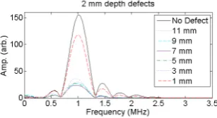
Example frequency content from some of the resulting signals can be seen in the fast Fourier transforms (FFTs) in figure 13 for defects of depth 2 mm. There is significant transmission around the 1 mm defect, but for the longer defects a near-constant frequency content is measured. The shape of the FFTs

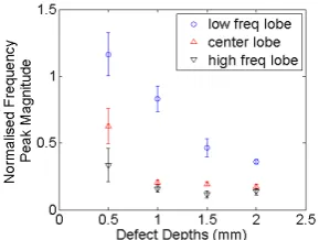
Figure 14: Relative change in frequency peak for the low frequency, center frequency, and high frequency lobes. The magnitudes were normalised to that for ‘no defect’.

are due to the finite width of the EMAT coil [22]. Analysis looked at the peak magnitudes in three of the frequency ‘lobes’; low frequency (0.35 - 0.67 MHz), main lobe (0.67 - 1.33 MHz), and high frequency (1.33 - 1.65 MHz).

The shortest defects, 1 mm and 3 mm, are very close to the size of the beam width, and so were excluded for calibration. The reference signal (no defect) was used to normalise the data, with the peak magnitude in each frequency region plotted as a function of depth in figure 14 following averaging of the data from the 5-11 mm length defects. As expected, all of the frequency peaks are increasingly attenuated with increasing defect depth. The high frequency lobe shows the most attenuation, while the low frequency has the least relative attenuation.

5. Orientation Variations

With some types of defect and sample the mechanism that causes the defect also dictates the orientation of its growth. However, this is not always the case. If the transducer happens to be orientated end on to a narrow, crack-like defect it may not detect it, even if the defect has significant spatial extent in the other dimensions. One solution is to perform at least two scans with the transducer rotated 90◦ between scans to ensure that reflections or changes in transmission are achieved, and improve the chances of a favorable orientation. This is, however, a time consuming solution, especially as for full coverage more than two orientations are necessary.

Figure 15: Four coil ring EMAT schematic. The magnetic field is orientated in to the plane of the paper.

the effect of crack orientation on the signals on each of the three detector coils. A 1 MHz driving frequency was used in this case for improved signal strength. The scanning set up is shown in figure 16, with 0◦defined as having the wave propagation direction parallel to the defect. The blue arrows represent some of the expected wave paths. Detector 2 will show full signal transmission at 0◦ and 180◦ as it is end on to the narrowest part of the defect, but will lose signal gradually until the detected signal is at its weakest at 90◦, when the longest extent of the defect is across the beam width. Detectors 1 and 3 should not receive any transmission, however, when the propagation direction is at 45◦ to the defect, detector 1 should pick up a reflection. It is also possible that there will be some diffraction from the defect. After 90◦ the signals should repeat, only with detectors 1 and 3 switched over.

The signal power measured by the three different detector coils is plotted in figure 17 as a function of orientation angle. Part (a) shows the data as a B-scan with the colour scaling showing normalised signal power from 0 (blue) to 1 (red), the x-axes show the signal arrival time, and the y-axes show the angle of rotation. Part (b) shows the maximum signal detected during a time window of 15-18 µs, matching the predicted arrival times of Rayleigh waves from the defects, plotted as a function of angle.

The data from each detector has been individually normalised. The trans-mitted signals measured by detector 2 are much stronger than the reflection / diffraction signals measured by detectors 1 and 3. For reference, the maximum signal in the raw data for each scan is 17.5, 67.1, and 16.3 mV for detectors 1, 2 and 3 respectively.

Figure 16: Rotational scan set up. The blue arrows indicate the expected wave paths.

strongest signals measured by detectors 1 and 3, arriving at around 45◦ for detector 1 and 135◦for detector 3, are Rayleigh wave reflections from the defect, while the weaker signals, appearing at around 135◦ for detector 1 and 45◦ for detector 3, are likely due to reflection or tip diffraction from the defect end.

Similarly to the length measurements, the exact angular ranges over which a defect is detectable is dependent upon how much signal variation is classed as significant. Using the 0.7 power level drop used previously for length gauging (corresponding to a drop in the signal power from 1 to 0.3), the transmitted signals give a detectable defect over a 70◦ range centred on 90◦. Using a 0.5 power level drop increases this range to 87◦, but this is still not sufficient to give detection over a wide range of orientations. Reducing the power level drop further will give a better range, and the 0.7 calibration was for accurate measurements rather than detectability, but will be liable to higher false calls.

Even within these detectable ranges for detector 2, the signal drop will not reflect the true severity of the defect except close to 90◦, but considering also the information from the side detectors will indicate if the defect severity is greater than measured. The signals measured by detectors 1 & 3 can increase the angular detection range for detectability by applying a further constraint on the level of the reflected signal; for example, by defining a power level of 0.3 as being sufficient to identify a defect, the range of detectability is increased to 16◦ to 170◦over the range from 0◦to 180◦. This is sufficiently above the noise level to indicate that signals are reliably being detected, and in practice one would set a threshold above which an indication is given, to remove the requirement for normalisation.

A full implementation of the technique would use the identical nature of the coils and multiplexing to alternately employ two of the coils which are located next to each other as generation coils, effectively rotating the data in figure 17 by 90◦. This multiplexing would remove the need for full rotation as well as linear scanning, enabling a simplified measurement system which is able to detect all orientations of defect. This could be combined with full rotational measurements once a defect is found, to ensure an accurate depth measurement using the transmitted waves.

6. Conclusion

of, a set of machined slot defects, down to 0.5 mm depth, 1 mm length, with an accuracy on the length measurements of ±0.4 mm after calibration. With a 1 MHz driving signal, transmission under the same machined slot defects indicated that the coil set up can be used for defect depth measurements, with the potential to use the defect depth effect on transmitted frequency for a reliable depth measurement. A set of four focused coils arrayed around the focal point was shown to significantly increase the ability to pick up defects at unknown orientations to the wave propagation direction. Defects were only undetectable over a very small angle range, and the use of multiplexing to use two coils alternately as the generation coil would enable detection of all orientation defects without the requirement for a rotational scan.

7. References

[1] S. L. Grassie, Wear2581310–1318 (2005)

[2] F. Hernandez-Valle, A. R. Clough and R. S. Edwards, Corrosion Science

78 335–342 (2014)

[3] C. B. Thring, Y. Fan and R. S. Edwards, Non-Destructive Testing and Evaluation International81 20–27 (2016)

[4] R. S. Edwards, S. Dixon and X. Jian, Ultrasonics441 93–98 (2006)

[5] R. J. Blake and L. J. Bond, Ultrasonics 28214–228 (1990)

[6] S. Boonsang and R. J. Dewhurst, Applied Physics Letters 82 3348–3350 (2003)

[7] R. S. Edwards, S. Dixon and X. Jian, Journal of Physics D: Applied Physics

37(16) 2291–2297 (2004)

[8] R. S. Edwards, X. Jian, Y. Fan and S. Dixon, Applied Physics Letters87

194104 (2005)

[9] J. L. Rose, Ultrasonic Waves in Solid Media,Cambridge University Press, Cambridge(1999)

[10] L. J. Bond, Ultrasonics1771–77 (1979)

[11] M. Hirao and H. Ogi, EMATs for Science and Industry: Noncontacting Ultrasonic Measurements, Kluwer Academic Publishers, Boston(2003)

[12] I. Baillie, P. Griffith, X. Jian and S. Dixon, Insight49(2) 87–92 (2006)

[13] S. B. Palmer and S.Dixon, Insight45211–217 (2003)

[14] A. S. Murfin, R. A. J. Soden, D. Hatrick and R .J. Dewhurst, Measurement Science and Technology111208–1219 (2000)

[16] W. A. K. Deutsch, A. Cheng and J. D. Achenbach, IEEE Transactions on Ultrasonics, Ferroelectrics, and Frequency Control 2A333–340 (1983)

[17] S. Dixon, T. Harrison, Y. Fan and P. A. Petcher, Journal of Phyics D: Applied Physics45175103 (2012)

[18] T. Stratoudaki, J. A. Hernandez, M. Clark and M. G. Somekh, Measure-ment Science & Technology 18843-851 (2007)

[19] T. Takishita, K. Ashida, N. Nakamura, H. Ogi and M. Hirao, Japanese Journal of Applied Physics5407HC04 (2015)

[20] American Society for Testing and Materials, Standard practice for ul-trasonic examinations using electromagnetic acoustic transducer (EMAT) techniques, (1996) Designation: E 1816 - 96

[21] C. B. Thring, Y. Fan and R. S. Edwards, Review of Progress in QNDE; submitted (2016)