warwick.ac.uk/lib-publications
Original citation:
Shadmehr, Mehdi and Bernhardt, Dan. (2017) Monotone and bounded interval equilibria in a coordination game with information aggregation. Mathematical Social Sciences, 89. pp. 61-69.
Permanent WRAP URL:
http://wrap.warwick.ac.uk/88532
Copyright and reuse:
The Warwick Research Archive Portal (WRAP) makes this work by researchers of the University of Warwick available open access under the following conditions. Copyright © and all moral rights to the version of the paper presented here belong to the individual author(s) and/or other copyright owners. To the extent reasonable and practicable the material made available in WRAP has been checked for eligibility before being made available.
Copies of full items can be used for personal research or study, educational, or not-for-profit purposes without prior permission or charge. Provided that the authors, title and full bibliographic details are credited, a hyperlink and/or URL is given for the original metadata page and the content is not changed in any way.
Publisher’s statement:
© 2017, Elsevier. Licensed under the Creative Commons Attribution-NonCommercial-NoDerivatives 4.0 International http://creativecommons.org/licenses/by-nc-nd/4.0/
A note on versions:
The version presented here may differ from the published version or, version of record, if you wish to cite this item you are advised to consult the publisher’s version. Please see the ‘permanent WRAP URL’ above for details on accessing the published version and note that access may require a subscription.
Monotone and Bounded Interval Equilibria in a
Coordination Game with Information Aggregation
1
Mehdi Shadmehr
2Dan Bernhardt
31We thank Raphael Boleslavsky, Ethan Bueno de Mesquita, Odilon Camara, Juan Carrillo,
Sylvain Chassang, Ehud Kalai, Tom Palfrey, Kris Ramsay, Kevin Reffett, and Stephen Morris for helpful suggestions. This note was originally part of a working paper “Coordination Games with Information Aggregation.”
2Department of Economics, University of Calgary, 2500 University Dr., Calgary, AB, T2N 1N4,
Canada. E-mail: [email protected]
3Department of Economics, University of Warwick and University of Illinois, 1407 W. Gregory
Abstract
We analyze how private learning in a class of games with common stochastic payoffs affects the form of equilibria, and how properties such as player welfare and the extent of strategic miscoordination relate across monotone and non-monotone equilibria. Researchers typically focus on monotone equilibria. We provide conditions under which non-monotone equilibria also exist, where players attempt to coordinate to obtain the stochastic payoff whenever sig-nals are in a bounded interval. In bounded interval equilibria (BIE), an endogenous fear of miscoordination discourages players from coordinating to obtain the stochastic payoff when their signals suggest coordination is most beneficial. In contrast to monotone equilibria, expected payoffs from successful coordination in BIE are lower than the ex-ante expected payoff from ignoring signals and always trying to coordinate to obtain the stochastic pay-off. We show that BIE only exist when, absent private information, the game would be a coordination game.
1
Introduction
In this paper, we analyze how private learning in a class of coordination games with common stochastic payoffs affects the nature and structure of equilibria, and how properties such as player welfare and the extent of strategic miscoordination are related across the monotone and non-monotone equilibria that may result. We analyze the game in Figure 1, where h,
l and w are known parameters with h > l, but θ is an unknown common stochastic payoff drawn from a distribution with supportR, and players receive noisy private signals aboutθ.
player A
player B
0 1
0 h, h w, l
1 l, w θ, θ
Figure 1
The game captures some key aspects of strategic interactions in a variety of economic and political settings. For example, it describes:
• A coup game between officers who must decide whether to mount a coup based on pri-vate signals about the successful coup payoff θ, where the coup only succeeds if both officers act. If one officer acts, the coup fails, and the disloyal officer is punished. The setting captures the possibilities that, when a coup fails, the loyal officer’s payoff can fall (w < h) if the ruler increases surveillance of the military or reduces its budget to weaken it; or it can rise (w > h) when a loyal officer who informs the ruler is rewarded, or the ruler raises the military budget to keep officers happy.1
• A technology adoption game in which firms must decide whether to stick to an existing platform or to pursue a new network/platform investment (with uncertain value) that
1Shadmehr and Bernhardt (2011) analyze monotone equilibria in a revolution setting in which citizens
only pays off if broadly adopted.
• A “relationship game” in which individuals, who know the value of their relationships with their current partners, receive signals about their payoffs if they break those re-lationships to form a new one together (action 1), where h > l reflects that breaking an existing relationship is costly if a potential partner does not reciprocate.
• A tariff war, in which countries choosing between high tariffs and free trade, where the countries know the payoffs from high tariffs, but receive signals about the uncertain political economy payoffs of free trade.
In these settings, the noisy signals typically leave players very uncertain about whether the actual payoffs from “successful” coordination on action 1 exceed the sure payoffs from coordinating on action 0, and the other player’s equilibrium action will contain material infor-mation about θ—players face both information aggregation and miscoordination concerns.2
Wereθ public information, then whenθ ≥w, equilibrium imposes no restrictions on how players coordinate: if a player believes the other will take action 1, then she will take action 1 to receiveθ; but if she believes that the other will take action 0, the miscoordination cost
µ≡h−l >0 causes her to take action 0, expecting only to receiveh. Concerns about strate-gic miscoordination can induce players to take action 0, no matter how highθ is. However, in most strategic settings, rather thanθbeing public information, players instead receive private noisy signals, leaving substantial uncertainty about its value. In such settings, we ask: what forms can equilibria take, and how do the properties of these equilibria relate to each other? Researchers typically focus on equilibria in finite-cutoff strategies in which a player takes action 0 when her signal aboutθis below some critical cutoff, but takes action 1 when the sig-nal is above. We show that such equilibria exist if and only ifµis sufficiently small.3 We then
provide conditions under which non-monotone equilibria also exist in which each player takes action 1 if and only if her signal is in a bounded interval. In these bounded interval equilibria (BIE), an endogenous fear of miscoordination discourages players from coordinating on ac-tion 1 to obtainθexactly when their signals suggest that coordination is most beneficial. We
2Chassang and Padr´o i Miquel (2010) analyze a related setting in which signal noise is vanishingly small,
so that only miscoordination concerns are present, and a unique monotone equilibrium obtains.
prove that bounded interval equilibria exist onlywhenfinite-cutoff equilibria exist, and that if, following a signal, a player takes action 1 in a bounded interval equilibrium, then she also does so in the largest finite-cutoff equilibrium. Moreover, bounded interval equilibria only exist if w < E[θ]—there must be sufficient potential surplus from coordinating on action 1. Thus, for bounded interval equilibria to exist, absent private information, the game must be a coordination game with bothh > landE[θ]> w. This means that in our private information setting, in any bounded interval equilibrium, players face an expected risk of miscoordination even when taking the “safe” action 0: unconditionally, were the other player to always take action 1, it must be better to always take action 1 than to always take action 0. We then highlight the bad welfare properties of bounded interval equilibria, showing that while in any finite-cutoff equilibrium, a player’s ex-ante expected payoff fromsuccessfullycoordinating on action 1 always exceeds E[θ], in any bounded interval equilibria, the opposite must hold.
We first analyze monotone equilibria. Given an affiliation assumption on signal structures plus some tail restrictions on distributions, we show that equilibria in finite-cutoff strategies exist if and only if the miscoordination costµis not too high. We then investigate the num-ber of finite-cutoff equilibria that can exist. Previous results based on additive normal noise signal structures suggest that generically either zero or two finite-cutoff equilibria exist—see footnote 1. We show that this result does not generalize. For example, with an additive logistic noise signal structure, a unique finite-cutoff equilibrium obtains whenµ is small.
We then ask whether and when more limited coordination can emerge in equilibrium. We search for equilibria in bounded interval strategies (BIS) in which players take action 1 whenever their signals about the common coordination payoff are high, but nottoohigh, i.e., whenever signals are inside a bounded interval (kL, kR). In such bounded interval equilibria
(BIE),4 a self-fulfilling fear of miscoordination causes players not to take action 1 precisely
when their signals suggest that the payoff from coordinating on action 1 is highest.
We first use Karlin’s variation diminishing theorem to show that when the conditional pdf of signals given θ is totally positive of order three (T P3), then the best response to a
BIS is either a BIS or always to take action 0. We next establish necessary and sufficient conditions for an arbitrary BIS (kL, kR) to be supported as an equilibrium for some set of 4By a bounded interval equilibrium, we mean an equilibrium in bounded interval strategies. We use BIE
primitive payoff parameters, {w, µ}: player indifference at kL and kR means that they must
be more likely to succeed in coordinating on action 1 following signal kL than signal kR,
since the expected payoff from successful coordination is higher givenkR.5
We show that if a bounded interval equilibrium (BIE) exists, then so does a finite-cutoff equilibrium. Moreover, any BIE must be “contained” in the largest monotone equilibrium— lettingk be the cutoff for the monotone equilibrium in which players take action 1 the most, we establish that k < kL, i.e., players are strictly more likely to take action 1 in the k
equilibrium. Intuitively, the finite-cutoff k equilibrium offers the promise of a better upside from coordination—the other player may have a really high signal—and miscoordination is less likely, making it worthwhile to risk trying to coordinate on action 1 following a less promising signal. We then show that if multiple finite-cutoff equilibria exist, and ¯k is the cutoff for the smallest one, thenkL <k¯: miscoordination is more likely following signal ¯k in
the monotone equilibrium than it is following signal kL in the BIE; but the potentially high
payoff if the other player has an especially high signal makes it worthwhile.6
To illustrate the extent to which the endogenously-generated fear of miscoordination must
necessarilybe severe in a BIE, we specialize to the classical additive normal noise signal struc-ture. Normalizing E[θ] = 0, we show that if (kL, kR) is a BIE, then kL < 0 and |kL| > kR,
implying that k < kL < kR <−k. Thus, on average, in a BIE, a player seeks to coordinate 5Chen and Suen (2015) investigate a game with model uncertainty where individuals update from their
incomes about whether a revolution would lead to an improved distribution of incomes. Equilibria take a bounded interval form, because wealthy individuals do not want to have their income re-allocated and hence have dominant strategies not to revolt; and poor individuals are pessimistic about the prospect that an improved distribution of incomes would result (and revolution is costly). From a technical perspective, Chen and Suen prove the existence of bounded interval equilibria using Tarski’s fixed point theorem. In contrast to our setting, in their setting, monotone equilibria do not exist (reflecting that the very poor and very rich never revolt), the best response to a BIS is always a BIS, the best response to a larger BIS is also a larger BIS (best responses are monotone with respect to set inclusion order), and one can construct a natural complete lattice consisting of non-degenerate intervals that the best response correspondence maps into itself. Therefore, Tarski’s theorem applies. However, in our setting, the best response to a BIS can be a monotone strategy. Moreover, when BIS is sufficiently large (with lower bound above that for the largest monotone equilibria), iterating on best responses can generate consecutively larger BISs (each containing the preceding one, implying a monotone mapping), but one cannot construct a complete lattice because each interation makes the resulting BIS closer to a monotone strategy, as the upper end of the BIS grows without bound. This means that one cannot apply Tarski’s theorem, necessitating a completely different approach to establishing the existence of a BIE.
6Because this game is not supermodular, one cannot invoke the result that the largest and smallest
to receiveθ on a very limited set of signals, and the expected fruits of such coordination are low relative to the potential benefits: conditional on coordinating on action 1 and obtaining
θ, a player’s expected payoff is lower than E[θ] = 0 in any BIE, while it is higher than E[θ] in any finite-cutoff equilibrium. Moreover, we show that for a BIE to exist, w must be less than E[θ]—BIE exist only when, absent private information, we have a coordination game. We conclude with a discussion of non-monotone equilibria, (a) when stochastic payoffs from coordinating on action 1 are private rather than common values; and (b) in global games that feature two-sided limit dominance (see e.g., Morris and Shin (2003)).
2
The Model
Two players A and B must choose between actions 0 and 1. Payoffs are depicted in Figure 1; players receive the common stochastic payoff θ if and only if they both take action 1, and payoffs h, l and w are common knowledge, with h > l. Each player i ∈ {A, B} receives a private signal si about θ. After receiving signals, players simultaneously take actions.
The signals and θ are jointly distributed according to a strictly positive, continuously differentiable density f(θ, sA, sB) on
R3. Players are symmetrically situated in the sense
that the signals are exchangeable, i.e., f(θ, s, s0) = f(θ, s0, s), for allθ, s, s0. We assume that
sA, sB and θ are strictly affiliated:7 a higher signal si represents good news about sj and θ. We also impose standard additional structure on the tail properties of f(θ, sA, sB):
Assumption A1 For i, j ∈ {A, B} with i6=j:
(a) lim
si→−∞P r(s
j > k|si) = 0 and lim si→∞E[θ|s
j > k, si] =∞, for all k ∈
R.
(b) lim
k→−∞E[θ|s
j > k, si =k] =−∞ and lim k→∞P r(s
j > k|si =k) E[θ|sj > k, si =k]<∞.
Assumption A1 implies that limk→∞P r(sj > k|si = k) = 0 and limsi→−∞E[θ|si] = −∞.
In the Online Appendix, we show that A1 holds with an additive noise signal structure,
si =θ+νi, where θ and νis are independent normal or logistic random variables.
A pure strategy for player iis a functionρi mapping her signalsi about θ into an action 7si, sj and θ are strictly affiliated if, for all z, z0 ∈
R3, with z 6= z0, f(min{z, z0})f(max{z, z0}) >
choice. That is, ρi :R→ {0,1}, where ρi(si) = 1 indicates that player i takes action 1, and
ρi(si) = 0 indicates that i takes action 0.
2.1
Monotone Equilibria
We first analyze monotone strategies, where a player’s strategy is (weakly) monotone in her signal. With finite-cutoff strategies, a playerj’s strategy is summarized by a critical cutoffkj:
ρj(sj) = 1 if sj > kj and ρj(sj) = 0 if sj ≤kj.
Let ∆(si;kj) be player i’s expected net payoff from taking action 1 rather than 0, given
her signal si and the other player’s cutoff kj. Then,8
∆(si;kj) =P r(sj > kj|si) (E[θ|sj > kj, si]−w)−P r(sj ≤kj|si) µ, (1)
whereµ≡h−l >0 is the net miscoordination cost of taking action 1 when the other player takes action 0. Playeri takes action 1 if and only if ∆(si;kj)>0.9
Because the payoff θ from coordinating on action 1 can be very low, the game is not supermodular. When player j reduces her cutoff kj (takes action 1 more), player i is less
likely to pay the miscoordination cost, i.e.,P r(sj ≤kj|si)µfalls, raisingi’s incentive to take
action 1, creating a force for strategic complements. However, when player j reduces her cutoffkj, playeri’s expected payoff from successful coordination on action 1, E[θ|sj > kj, si],
alsofalls, reducing her incentive to take action 1, creating a force for strategic substitutes. Always taking action 1 is never a best response. To see this, first note that if player j
always takes action 1, then playeritakes action 1 if and only ifE[θ|si]> w, andA1implies limsi→−∞E[θ|si] = −∞ < w. Next, note that if, instead, player j adopts a finite-cutoff
strategy with cutoff kj, then from equation (1),
lim
si→−∞∆(s
i;kj) = lim
si→−∞P r(s
j > kj|si) (E[θ|sj > kj, si]−w)−P r(sj ≤kj|si) µ <0,
since limsi→−∞E[θ|sj > kj, si] < ∞ and limsi→−∞P r(sj ≤ kj|si) = 1 from A1. Thus, i
takes action 0 if her signal is sufficiently low. Further, since h > l, if player j always takes
8Throughout the paper, we assume the existence of the expectations that we use.
9To ease exposition, we assume that in the non-generic event that a player is indifferent between taking
action 0, then so should player i: always taking action 0 is always an equilibrium. Besides this equilibrium, all other monotone equilibria are in finite-cutoff strategies. Unless stated otherwise, in what follows, when we write a cutoff strategy, we mean a finite-cutoff strategy. Lemma 3 in the Appendix establishes that the best response to a finite-cutoff strategy is a unique finite-cutoff strategy. Thus, a pair of finite cutoffs (ki, kj) is an equilibrium if
and only if ∆(ki;kj) = ∆(kj;ki) = 0. Throughout, we focus on symmetric equilibria where
kj =ki =k. Thus, (k, k) is a (symmetric) cutoff equilibrium if and only if ∆
1(k) = 0, where
∆1(k)≡∆(k;k) =P r(sj > k|si =k) (E[θ|sj > k, si =k]−w+µ)−µ. (2)
We say that a cutoff equilibrium is larger when its cutoff is smaller, so that players are more likely to take action 1 in that equilibrium. Proposition 1 characterizes cutoff equilibria.
Proposition 1 There exists a threshold µ∗ >0 on miscoordination costs such that a finite-cutoff equilibrium exists if µ < µ∗, but not if µ > µ∗.10 Moreover, if ∆1(x) is either
single-peaked or strictly increasing, then at most one other finite-cutoff equilibrium exists.
Proposition 1 reveals that when the miscoordination cost µis large, the potential gains from coordinating on action 1 and obtaining θ are swamped by the risk of taking action 1 when the other player takes action 0. One might posit that as µrises and incentives to take action 1 fall, equilibrium cutoffs could adjust, preserving finite-cutoff equilibria. However, because the expected value of coordinating on action 1 is bounded from above (by A1 (b)), sufficiently high miscoordination costsµ always swamp the possible coordination gains.
The properties of best response curves provide further insights. Let ki(kj) be player i’s
unique best response cutoff to player j’s cutoff kj. Even were j to always take action 1,
player ionly takes action 1 when her signal is sufficiently high, i.e., limkj→−∞ki(kj) is finite.
Thus, if ki(kj) crosses the 45◦ line, the first crossing must occur from above. Moreover,
raising the punishment cost µ or the predatory payoff w makes a player more hesitant to take action 1, i.e.,ki(kj) shifts upward, ∂ki∂µ(kj;µ), ∂ki(∂wkj;w) >0. Once the miscoordiantion cost
µ exceeds a threshold, ki(kj) > kj for all kj, and hence no finite-cutoff equilibrium exists. When µ is below that threshold, at least one finite-cutoff equilibrium exists.
When ∆1(x) is single-peaked or strictly increasing, there can be at most two finite-cutoff
equilibria. In the Online Appendix, we show that whensi =θ+νi, (1) if θ andνis are inde-pendent normal random variables, then ∆(x) is single-peaked for all µ > 0 and w; and (2) if θ, νA, νB ∼ iid e−x
(1+e−x)2 (logistic), then ∆(x) is single-peaked when µ is large enough that
w <1+µ, but is strictly increasing whenw≥1+µ. We also provide alternative general suffi-cient conditions for ∆1(k) to be single-peaked or increasing: (1)P r(sj > k|si =k) is
decreas-ing and logconcave ink, and (2)E[θ|sj > k, si =k]−w+µis logconcave ink when positive.
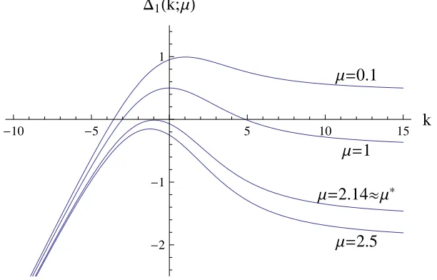
Let k be the cutoff for the largest finite-cutoff equilibrium, and ¯k be the cutoff for the smallest finite-cutoff equilibrium when multiple equilibria exist. Because raisingµorwshifts ∆1(k) downward, when ∆1(x) is single-peaked or strictly increasing, increases inµorwraise
k, but reduce ¯k: the largest finite-cutoff equilibrium has “natural” comparative statics, but the smallest one has the opposite comparative statics, reflecting that it is locally unstable.
Μ=0.1
Μ=1
Μ=2.14»Μ*
Μ=2.5
-10 -5 5 10 15 k
-2 -1 1
D1Hk;ΜL
Figure 2: ∆1(k;µ) as a function of k for different values of miscoordination costs µ.
si = θ+νi, i ∈ {A, B}, where θ and νis are iid logistic e−x
(1+e−x)2. When µ is small, there is
a unique finite-cutoff equilibrium. Parameters: w=−1.5.
When ∆1(x) is single-peaked or strictly increasing, the right-tail properties of ∆1(k)
de-termines the number of finite-cutoff equilibria. With an additive normal signal structure, Shadmehr and Bernhardt (2011) show that limk→∞∆1(k)< 0, so either zero or two
[image:11.612.154.460.363.559.2]can be positive, implying a unique finite-cutoff equilibrium—see the Online Appendix.
2.2
Bounded Interval Equilibria
We next investigate when other types of equilibria can exist. In particular, we determine when an endogenously-generated fear of miscoordination can give rise to equilibria in which players sometimes seek to coordinate on action 1, but fail to do so precisely when their signals suggest that payoffs from successful coordination would be very high. We then relate the properties of monotone and these non-monotone, bounded interval equilibria (BIE), and characterize the primitive parameters for which BIE do and do not exist.
We say that player j adopts the bounded interval strategy (kLj, kjR) when
ρj(sj) = 1 if and only if kjL< s j < kj
R, with k j L, k
j
R∈R. (3)
Let Γ[si;kjL, kRj] be player i’s net expected payoff from taking action 1 when her signal is si
and player j adopts interval strategy (kLj, kjR). Mirroring the derivation of equation (1),
Γ[si;kLj, kRj] =P r(kLj < sj < kRj|si) (E[θ|kjL< sj < kRj, si]−w+µ)−µ. (4)
To characterize best responses to a bounded interval strategy (BIS), it helps to link Γ[si;kj L, k
j R]
to player i’s net expected payoff from taking action 1 if she knew θ. Let π(θ;kLj, kRj) be i’s incremental return from taking action 1 given θ and (kLj, kjR):
π(θ;kLj, kjR) = (θ−w) P r(kjL< sj < kRj|θ) + (l−h) (1−P r(kjL< sj < kRj|θ)) = (θ−(w−µ)) P r(kLj < sj < kRj|θ)−µ. (5)
Then we can write player i’s net expected payoff from taking action 1 given signalsi as
Γ(si;kLj, kjR) =
Z ∞
−∞
π(θ;kjL, kRj)f(θ|si)dθ, (6)
where f(θ|si) is the pdf of θ given si. To analyze the properties of Γ(si;kj L, k
j
R), we use
Karlin’s theorem on the variation diminishing property of totally positive functions (Karlin 1968, Ch. 1, Theorem 3.1). A functionK(x, y) is Totally Positive of ordern,T Pn, whenever
K(x, y) ∂
∂yK(x, y) · · ·
∂m−1
∂ym−1K(x, y) ∂
∂xK(x, y)
∂2
∂x∂yK(x, y) · · ·
∂m
∂x∂ym−1K(x, y)
..
. ... . .. ...
∂m−1
∂xm−1K(x, y)
∂m
∂xm−1∂yK(x, y) · · ·
∂2(m−1)
∂ym−1∂xm−1K(x, y)
From Karlin’s theorem, if K(si, θ) = f(θ|si) is totally positive of order n and π(θ) has
r ≤n−1 sign changes, then Γ(si;kLj, kjR) has at most r sign changes. We assume that our information structure has the following properties:
Assumption A2 For i, j ∈ {A, B}withi6=j, the probability density ofsi conditional onθ,
f(si|θ), is totally positive of order three (T P
3), andP r(kL < si < kR|θ)is strictly logconcave
in θ. Moreover, limsi→∞E[θ|sj, si]f(sj|si) = limsi→∞f(sj|si) = 0 for any sj.
We show in an Online Appendix that A2 holds if si = θ +νi, where θ and νis are in-dependent normal or iid logistic random variables.11 Given this structure, we use Karlin’s theorem to derive the shapes of Γ(si;kj
L, k j
R) and π(θ;k j L, k
j
R), using equations (4) to (6).
This allows us to characterize the best response to a BIS:
Lemma 1 Suppose player j adopts a bounded interval strategy. Then, either player i’s best response is a bounded interval strategy, or it is to always take action 0.
We first use logconcavity to show that (i) π(θ;kLj, kRj) has a unique maximum whenever it is positive, and (ii) when θ increases unboundedly, P r(kL < si < kR|θ) approaches zero
at a rate faster than exponential functions (An 1998), and hence limθ→∞P r(kL < si <
kR|θ)(θ−(w−µ)) = 0.We use these to show thatπ(θ;kjL, k j
R) has at most two sign changes.
We then use the fact that because f(si|θ) is T P
3, Karlin’s theorem implies that Γ(si;kLj, k j R)
has at most two sign changes. Moreover, limsi→±∞Γ[si;kLj, kjR] < 0.12 This implies that
either Γ[si;kLj, kjR] has two sign changes or no sign change, in which case it must be neg-ative. And, if Γ[si;kLj, kjR] has exactly two sign changes, then as si traverses from −∞ to
∞, Γ(si;kjL, kRj) must first change sign from negative to positive and then from positive to negative; this is precisely the property of a bounded interval strategy (BIS).
Throughout, we focus on symmetric BIE. The necessary and sufficient condition for (kL, kR) to be a symmetric BIE is Γ[si;kL, kR]>0 if and only ifsi ∈(kL, kR). To find a
sym-metric BIE, one must solve the system of equations that describe a player’s indifference be-tween taking actions 0 and 1 at the cutoffs: Γ[si =k
L;kL, kR] = 0 and Γ[si =kR;kL, kR] = 0. 11Supposeνi∼h. Then, affiliation (T P
2) requireshto be log-concave: (h0)2≥hh00. T P3 involves higher
derivatives ofh, in particular, ∂∂s3f(si∂i2|θθ) =−
∂3f(si|θ) ∂2si∂θ =h
(3)(si−θ) and ∂4f(si|θ) ∂2si∂2θ =h
(4)(si−θ).
12FromA2, (i) lim
si→∞E[θ|sj, si]f(sj|si) = 0, which implies limsi→∞P r(kL< sj < kR|si)E[θ|kL< sj<
kR, si] = limsi→∞R kR kL E[θ|s
j, si]f(sj|si) = 0; and (ii) lim
si→∞f(sj|si) = 0, which implies limsi→∞P r(kL<
Γ[kR;kL,kR]=0
Γ[kL;kL,kR]=0 Γ[kL;kL,kR]=0
(-9.98,-1.88)
(-0.63,-0.08) kL
kR
-μ
(-9.98,0) (-1.88,0)
-30 10 s
i
-4 2 Γ[si;k
[image:14.612.72.550.115.335.2]L,kR]
Figure 3: A bounded interval equilibrium. The left panel depicts contour curves Γ[kL;kL, kR] = 0, Γ[kR;kL, kR] = 0, and their intersections. The right panel depicts
Γ[si;k
L = −9.98, kR =−1.88]. The panels together show that (−9.98,−1.88) is a bounded
interval equilibrium. The numbers are two-decimal approximations. Parameters: w =−5,
µ= 1, and si =θ+νi, i∈ {A, B}, with θ, νA, νB ∼iidN(0,1).
These equations are only necessary conditions. To show that they are also sufficient, Lemma 2 shows that Γ changes sign at any solution of these equations. Therefore, any solution to these equations describes a BIE:
Lemma 2 (kL, kR) with kL, kR ∈ R and kL< kR is a bounded interval equilibrium strategy
if and only if Γ[kL;kL, kR] = 0 and Γ[kR;kL, kR] = 0.
Figure 3 illustrates an equilibrium in bounded interval strategies. Next, we determine for a given signal structure f(θ, sA, sB) that satisfies A1 and A2 and anarbitrary bounded interval strategy (kL, kR), whether there exist primitive payoff parameters {µ, w} that
sup-port (kL, kR) as an equilibrium. Proposition 2 details necessary and sufficient conditions for
(kL, kR) to be an equilibrium forsome set of primitives.
Proposition 2 There exist payoff parameters {µ, w} for which (kL, kR) is an equilibrium
BIS if and only if P r(sj ∈(k
L, kR)|si =kL)> P r(sj ∈(kL, kR)|si =kR), for i6=j.
symmet-ric equilibrium BIS, (kL, kR), are Γ[si = kL;kL, kR] = Γ[si = kR;kL, kR] = 0. Rearranging
these indifference conditions yields
µ = P r(kL< sj < kR|si =kL) (E[θ|kL < sj < kR, si =kL]−w+µ)
= P r(kL< sj < kR|si =kR) (E[θ|kL < sj < kR, si =kR]−w+µ).
A player with high signal si = k
R is more optimistic about the expected value of θ than if
she sees signal si =k
L. To be indifferent between taking actions 0 and 1 after both signals,
she must be more pessimistic about the likelihood of coordinating onθ given si =k
R. Thus,
P r(sj ∈(kL, kR)|si =kL)> P r(sj ∈(kL, kR)|si =kR).
The indifference conditions also shed light on the primitives that support (kL, kR) as a BIE.
Since P r(sj ∈(k
L, kR)|si =kL)<1, it must be that
E[θ|kL< sj < kR, si]−w+µ > µ, for si ∈ {kL, kR}.
Rearranging yields a bound on the predatory payoff w:
E[θ|kL< sj < kR, si]> w, for si ∈ {kL, kR}. (7)
The intuition is simple: player i is hurt when she takes action 1 rather than action 0 if
j takes action 0, receiving l rather than h. Thus, to be willing to take action 1, i must expect to gain from taking action 1 rather than action 0 if j instead takes action 1. This inequality also holds for all si > kR—were such a player to know that the other agent had
a signal sj ∈ (kL, kR), she would also want to take action 1 for higher signals; but she
as-signs such a low probability to the event sj ∈(kL, kR), and hence such a high probability to
miscoordination, that she chooses to take action 0 despite her high signal.
Properties of bounded interval equilibria. To characterize bounded interval equilibria, we next relate BIE and monotone equilibria. We then specialize to the classical additive normal noise signal structure to highlight the surprisingly strong structure that Proposition 2 places on the nature and extent of coordination that can occur in any BIE. Recall that
Proposition 3 If a BIE exists, then finite-cutoff monotone equilibria exist. If (kL, kR) is a
bounded interval equilibrium strategy, thenk < kL, i.e., players take action 1 following worse
signals in the largest finite-cutoff (k) equilibrium than in any BIE.
If limk→∞∆1(k) < 0 and a BIE exists, then multiple finite-cutoff monotone equilibria
exist. If (kL, kR) is a bounded interval equilibrium strategy, then kL < k¯, where ¯k is the
cutoff for the smallest finite-cutoff equilibrium.
The intuition comes from a decomposition of Γ[si =k
L;kL, kR]:
Γ[si =kL;kL, kR] =−P r(sj > kR|si =kL) (E[θ|sj > kR, si =kL]−w+µ) + ∆1(kL), (8)
where E[θ|sj > kR, si = kL]−w+µ > 0.13 A player must be indifferent between actions
0 and 1 when his signal just equals the lower cutoff kL of a BIE. Thus, when a player j
chooses the cutoff strategy kL instead of a BIS, so that j takes action 1 after receiving all
“better signals,” player ihas more incentive to take action 1 than in the BIE. In particular, where she was indifferent between actions (at si = k
L) in the BIE, she now strictly prefers
to take action 1: Γ[si = k
L;kL, kR] = 0 implies ∆1(kL) = ∆(si = kL;kL) > 0. Because
limk→−∞∆1(k)<0, there exists a cutoff k < kL at which ∆1(k) = 0.
If, in addition, limk→∞∆1(k) < 0, then there are multiple solutions to ∆1(k) = 0, i.e.,
there are multiple finite-cutoff equilibria. The largest such cutoff, ¯k exceeds kL: this follows
since ∆1(kL) > 0 but ∆1(k) < 0 for k > k¯. Moreover, because the gains from
success-ful coordination following signal ¯k in the cutoff equilibrium exceed those in the BIE given signal kL, the probability of successful coordination must be lower given ¯k than kL in the
corresponding equilibrium.
Corollary 1 Players are more likely to take action 1 in the largest finite-cutoff equilibrium than in any BIE.
When w > l, players take action 1 too little in thek equilibrium from a welfare perspec-tive (Shadmehr and Bernhardt (2015)), implying that BIE are welfare dominated.
Additive normal noise signal structure. To illustrate the sharp bite of the necessary condition in Proposition 2 that P r(sj ∈ (kL, kR)|si =kL) > P r(sj ∈ (kL, kR)|si = kR), we
13Note that (E[θ|sj > k
R, si = kL]−w+µ) > E[θ|kL < sj < kR, si =kL]−w >0, where the second
now specialize to the classical additive normal noise signal structure. The key structure that we exploit is that the signals shift the distribution, so that single-peakedness and symmetry are preserved and the dispersions of conditional distributions do not depend on signals.
Suppose si =θ+νi,i∈ {A, B}, where θ andνi’s are independent withθ ∼N(0, σ2) and
νi ∼N(0, σ2
ν). Letb ≡ σ2 σ2+σ2
ν, and recall that pdf(s
j|si) ∼ N(bsi,(1 +b)σ2
ν). First, observe
that when the noise in signals goes to zero, in the limit,P r(sj ∈(k
L, kR)|si =kL) =P r(sj ∈
(kL, kR)|si = kR) = 12, implying that BIE do not exist.14 Proposition 4 details the sharp
restrictions imposed on possible BIE using the fact that raising si from k
L to kR just shifts
the conditional distribution f(sj|si) to the right:
Proposition 4 If (kL, kR) is a bounded interval equilibrium strategy, then kL < E[θ] = 0
and |kL|>|kR|.
Recall that if (kL, kR) is an equilibrium BIS, a player i must be more pessimistic about
the likelihood of coordinating on θ given si = k
R: P r(sj ∈ (kL, kR)|si = kL) > P r(sj ∈
(kL, kR)|si =kR). With an additive normal noise signal structure, this inequality becomes
|bkL−(kL+kR)/2|<|bkR−(kL+kR)/2|. (9)
Inspection of (9) reveals that for it to hold, we must have kL<0 and|kL|>|kR|.
Corollary 2 Relative to finite-cutoff equilibria, coordination in BIE on action 1 is limited and it is on less promising values: In particular, k < kL < kR < −k, where k < 0 and
E[θ|kL< sj < kR, si =kL]<0.
The corollary highlights the severity of the endogenously-generated fear of miscoordination after high signals in any BIE. For a BIE to exist, we must have k < kL < 0; and k < 0
implies that in the finite-cutoff equilibrium supporting the most coordination on θ, players seek to coordinate on action 1 for a majority of signals. In contrast, in a BIE, players fail to coordinate following all good signalssi >−k.
14lim
σν→0P r(kL< s j< k
R|si=kL) = limσν→0Φ
kR−bkL √
(1+b)σ2
ν
−limσν→0Φ
(1−b)kL √
(1+b)σ2
ν
= 1−1 2 =
1 2, where
we use limσν→0 1−b √
(1+b)σ2
ν
= 0. Similarly, limσν→0P r(kL< s j< k
These results highlight that BIE have particularly bad welfare properties relative to finite-cutoff equilibria. In finite-finite-cutoff equilibria, a player’s expected payoff, given just her own information and conditional on successfully coordinating on action 1 to obtainθexceedsE[θ]:
Z ∞
k
E[θ|si] pdf(si|si > k) dsi > E[θ] = 0.
The fact that coordination succeeds only when the other player also has a good signal,sj > k
reinforces this. In sharp contrast, in BIE, |kL| > kR and kL < 0 imply that a player’s
ex-pected payoff, given just her own information and conditional on successfully coordinating on action 1 to obtain θ, is worse than E[θ]:
Z kR
kL
E[θ|si] pdf(si|si ∈(kL, kR))dsi < E[θ] = 0.
The fact that coordination only succeeds when the other player also has a signalsj ∈(kL, kR)
further reduces the expected payoff from ‘successful’ coordination in a BIE.
Because expected payoffs in BIE are lower than those for finite-cutoff equilibria, BIE cease to exist for lower miscoordination costs than for finite-cutoff equilibria:
Corollary 3 Recall that finite-cutoff equilibria exist whenever µ < µ∗. There exists a
µ∗∗< µ∗ such that ifµ > µ∗∗, then no bounded interval equilibrium exists.
Why then do BIE exist and when? Summarizing our previous results, recall that play-ers’ indifference at the bounds of an equilibrium BIS (kL, kR) has two implications. First,
equation (7) revealed that E[θ|kL < sj < kR, si = kL] > w. Second, Proposition 2 revealed
that P r(sj ∈ (kL, kR)|si = kL) > P r(sj ∈ (kL, kR)|si =kR), which Proposition 4 shows for
a normal-noise signal structure implies kL < 0 and |kL| > |kR|. These latter results imply
that E[θ|kL< sj < kR, si =kL]< E[θ] = 0. Combining these results yields:
Corollary 4 A necessary condition for a BIE to exist is w < E[θ] = 0.
is necessary for a BIE to exist highlights that there must be sufficient expected potential surplus from coordinating on action 1 to compensate for the facts that in a BIE, (i) players fail to coordinate on action 1 precisely when the payoff from doing so is expected to be high, thereby foregoing much of the benefits of coordinating on action 1; and (ii) a player is hurt when she tries to coordinate on action 1, but the other player does not.
In many of the economic settings described by the payoffs in Figure 1, the payoff hfrom coordinating on action 0 is less than the payoffwfrom taking action 0 when the other player takes action 1. For example, in an international trade game, the payoff when both countries set high tariffs is less than the payoff from setting a high tariff when the other country lowers its barriers. In such settings, the results in Corollary 4 are reinforced: BIE only exist when the status quo payoff of h (e.g., trade wars) is also low relative to the ex-ante expected benefits of coordinating on action 1 (e.g., free trade)—but the agents nonetheless get the low status quo payoff when signals about coordination are promising.
3
Discussion
A thorough analysis of non-monotone equilibria in a broader class of games is beyond the scope of our paper. However, it is straightforward to establish that BIE can exist in the private value analogue of our common value coordination setting, in which a player i’s ex-pected payoff when both players coordinate on action 1 is given by her signalsi. Indeed, the intuitions and qualitative properties that we have emphasized carry over directly.
One may also wonder if the one-sided limit dominance property15 of our game is
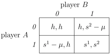
essen-tial for the existence of non-monotone equilibria. Clearly, in games featuring two-sided limit dominance, a bounded interval strategy is never a best response, and hence bounded interval equilibria cannot exist. Still, more complex non-monotone equilibria may exist. To see this, consider the classical private value investment game of Morris and Shin (2003) in Figure 4, where action 1 corresponds to invest and action 0 corresponds to not invest.
Clearly, no BIE exists because a player always takes action 0 when her signalsiis less than
h, and she always takes action 1, when her signal exceedsh+µ. The question is: can slightly
15A player has a dominant strategy to take action 0 if her signal is low enough, but does not have a dominant
player A
player B
0 1
0 h, h h, s2−µ
[image:20.612.218.394.109.196.2]1 s1−µ, h s1, s2
Figure 4: Private Value Game.
more complex non-monotone equilibria exist in which players take action 1 when their signals are either in a bounded interval or exceed a threshold, (k1, k2)∪(k3,∞) fork1 < k2 < k3 ∈R?
To show that such non-monotone equilibria can exist, we construct a non-monotone equi-librium for an additive normal noise signal structure,si =θ+νi, whereθ, νA, νB ∼iidN(0,1).
In such an equilibrium, players must be indifferent at the cutoffs, k1, k2 and k3. Defining
Ω≡(−∞, k1)∪(k2, k3), the indifference conditions are:
ki−P r(Ω|sj =ki) µ=h, i∈ {1,2,3}, j ∈ {A, B}.
In particular, we must have
k2−k1
P r(Ω|k2)−P r(Ω|k1)
= k3−k2
P r(Ω|k3)−P r(Ω|k2)
. (10)
Then (k1, k2, k3) = (k,0,−k) satisfies equation (10). For example, (k1, k2, k3) = (−5,0,5)
is supported as an equilibrium by µ = k2−k1
P r(Ω|k2)−P r(Ω|k1) ≈ 10.8986 and h = ki −P r(s 2 ∈
(−∞, k1)∪(k2, k3)|s1 =ki)×µ≈ −5.4493. Figure 5 illustrates that, for these parameters,
the non-monotone strategy (k1, k2, k3) = (−5,0,5) is the best response to itself, and hence
-10 -5 5 10 s i
[image:21.612.164.451.111.297.2]-6 -4 -2 2 4 6 Δ(si;(-5,0,5))
Figure 5: Net expected payoffs as a function of signal si given the other player’s
non-monotone strategy (k1, k2, k3) = (−5,0,5). Parameters: µ= 10.8986 and h=−5.4493.
4
Appendix: Proofs
Proof of Proposition 1: First, we prove a lemma.
Lemma 3 The best response to a finite-cutoff strategy is a unique finite-cutoff strategy.
Proof: Fix a finite cutoff kj. From equation (1), if ∆(si = x;kj) = 0, then (E[θ|sj >
kj, si = x]−w) ≥ 0; and by affiliation, both P r(sj > kj|si) and E[θ|sj > kj, si] increase
with si. Thus, if ∆(si =x;kj) = 0, then ∆(si;kj)>0 for all si > x. Furthermore, from A1 (a), limsi→−∞∆(si;kj) < 0 <limsi→+∞∆(si;kj). Thus, for every kj, there exists a unique
si =ki such that ∆(ki;kj) = 0. In addition, atsi =ki,
∂∆(si;kj)
∂si
si=ki
>0. (11)
Now, rewrite equation (2) as
∆1(k) = P r(sj > k|k) E[θ|sj > k, k]−P r(sj > k|k)w−(1−P r(sj > k|k))µ. (12)
For anyk, ∂∆1(∂µk;µ) =−(1−P r(sj > k|k))<0: raisingµuniformly lowers the curve ∆
1(k;µ).
Next, we show that when µ is sufficiently small, ∆1(k) crosses zero at least once; and
0) = P r(sj > k|k) (E[θ|sj > k, k]−w). E[θ|sj > k, si = k] increases in k by affiliation, and from A1, limk→±∞E[θ|sj > k, si = k] = ±∞. Therefore, for a given w, ∆1(k;µ = 0)
crosses zero from below—at a unique point. Thus, from the continuity of ∆1(k;µ) in k and
µ, ∆1(k;µ) = 0 has a solution for sufficiently small µ >0.
Lemma 4 There exists a µ >¯ 0 such that if µ >µ¯, then ∆1(k)<0 for all k.
Proof: Consider ∆1(k;µ) from equation (12), where we have made the dependence of ∆1
on the parameter µ explicit. First, observe that ∆1(k;µ) is uniformly decreasing in µ: for
any k, ∆1(k;µ1)> ∆1(k;µ2) for all µ2 > µ1. Thus, if for some µ= ˆµ, ∆1(k; ˆµ)< 0 for all
k, then ∆1(k;µ)<0 for all µ >µˆ. Now, suppose that the statement of the lemma is false.
Then, it must be the case that for all µ, there is some k such that ∆1(k;µ)≥0. We seek a
contradiction.
From A1 (b), limk→−∞E[θ|sj > k, k] = −∞, and hence limk→−∞∆1(k;µ) < 0 for all
µ > 0. Recall our premise that, for all µ, there is some k such that ∆1(k;µ) ≥ 0. Thus,
because ∆1(k;µ) is continuous in k, there exists a smallest k ∈ R at which ∆1(k;µ) ≥ 0.
Call it k(µ)∈R, and observe that k(µ) is weakly increasing in µ. LetM(µ)≡supk∈[k(µ),∞)P r(sj > k|k)E[θ|sj > k, k] andm(µ)≡inf
k∈[k(µ),∞)(1−P r(sj >
k|k)). Clearly,
∆1(k;µ)≤M(µ) +|w| −m(µ) µ.
Because k(µ) is weakly increasing in µ,M(µ) is weakly decreasing inµ and m(µ) is weakly increasing in µ. Moreover, from A1 (b), limk→∞P r(sj > k|k) E[θ|sj > k, k] < ∞, i.e., P r(sj > k|k)E[θ|sj > k, k] is bounded from above, and henceM(µ) is bounded from above.
Further, A1 (b) implies that limk→∞(1−P r(sj > k|k)) = 1. Because this limit is strictly
positive and f(θ, sA, sB) has full support by assumption, m(µ)>0. Recalling that M(µ) is weakly decreasing inµandm(µ) is weakly increasing inµ, we have,M(µ)+|w|−m(µ)µ <0 for sufficiently largeµ. Since ∆1(k;µ)≤M(µ) +|w| −m(µ) µ, then forµsufficiently large,
we have ∆1(k;µ)<0 for allk, a contradiction.
Therefore, there exists aµ∗ >0 such that ∆1(k) = 0 has a solution if µ < µ∗ and it does
not have a solution if µ > µ∗. It is immediate that when ∆1(k) is either single-peaked or
Proof of Lemma 1. We proceed in two steps.
Step 1: We show that π(θ;kLj, k j
R), from equation (5), has at most two sign changes.
Ob-serve that [θ−(w−µ)]P r(kjL< sj < kRj|θ) has a unique root atw−µ. Let g(θ)≡P r(kLj < sj < kj
R|θ). Differentiating [θ−(w−µ)] P r(k j
L< sj < k j
R|θ) with respect to θ yieldsg(θ) +
[θ−(w−µ)]g0(θ). Thus,g(θ)+[θ−(w−µ)]g0(θ)>0 if and only ifg(θ)>−[θ−(w−µ)]g0(θ). If θ > w−µ, this inequality is equivalent to − 1
θ−(w−µ) < g0(θ)
g(θ). The left-hand side is strictly
increasing in θ and the right-hand side is strictly decreasing because g(θ) is logconcave by
A2. Thus, they can cross at most once, in which case the intersection identifies a local maxi-mum. Next, observe that [θ−(w−µ)]g(θ) = 0 atθ =w−µ, and limθ→∞[θ−(w−µ)]g(θ) = 0
from log-concavity (An 1998, Corollary 1). Thus, the crossing, indeed, happens exactly once. That is, (θ−(w−µ)) P r(kLj < sj < kjR|θ) has a unique maximum forθ ∈ (w−µ,∞), and is negative for θ ∈(−∞, w−µ). Since π(θ;kLj, kRj) equals (θ−(w−µ))P r(kjL< sj < kRj|θ) minus µ >0, it inherits the shape, and has at most two sign changes (see Figure 3).
Step 2: Step 1 shows thatπ(θ;kLj, k j
R) has at most two sign changes. Now, consider equation
(6), and recall thatA2 implies that f(θ|si) is T P
3. Thus, by Karlin’s theorem, Γ(si;kLj, k j R)
has at most two sign changes. Footnote 12 shows that limsi→±∞Γ[si;kLj, kjR] <0. Thus, (i)
Γ(si;kj L, k
j
R) has either no sign change or two sign changes, (ii)if it has no sign change, then
Γ(si;kLj, kjR) < 0 for all si, i.e., player i never takes action 1, and (iii) if Γ(si;kjL, kRj) has two sign changes, then as si traverses R from −∞ to∞, Γ(si;kLj, kRj) is first negative, then positive, and then negative, which implies a bounded interval strategy.
Proof of Lemma 2: The “only if” part is immediate from the continuity of Γ[si;kL, kR] in
si for i∈ {A, B}. Next, we prove the “if” part. If Γ[si;k
L, kR] changes sign at bothkL and
kR, then from Lemma 1, Γ[si;kL, kR]>0 if and only if si ∈(kL, kR). Otherwise, Γ does not
change sign at kL or kR or both. We consider two cases:
Case I: Suppose Γ changes sign at only one of kL and kR. WLOG, suppose Γ changes
sign at kR, but not kL. Then kL must be a local maximum (minimum). Adding a small
positive (negative) constant toπ in equation (6) adds a constant to Γ,
Z ∞
θ=−∞
(π(θ;kLj, kjR) +)f(θ|si)dθ = Γ(si;kLj, kRj) +,
and hence createskLl and kLr at which Γ +changes sign, with kLl < kL < kLr < kR. Thus,
the proof of Lemma 1, π+ has at most two sign changes, which together with the T P3
property off(θ|si) implies that Γ +has at most two sign changes, which is a contradiction. Case II: Suppose Γ does not change sign at kL and kR. If kL and kR are both local
max-ima or both local minmax-ima, an argument similar to Case I leads to a contradiction. If one is a local maximum and the other is a local minimum, then there exists akM withkL< kM < kR
at which Γ changes sign. Now apply the argument in Case I with kM instead of kR. Proof of Proposition 2: From Lemma 2, (kL, kR) is a symmetric bounded interval
equi-librium strategy if and only if Γ[kL;kL, kR] = Γ[kR;kL, kR] = 0. Solving for−wfrom (4) and
using the notation in (3), yields
−w= µ
P r(ρj = 1|si =kL)
−µ−E[θ|kL, ρj = 1] =
µ
P r(ρj = 1|si =kR)
−µ−E[θ|kR, ρj = 1],
(13) where E[θ|z, ρj = 1] means E[θ|si =z, ρj = 1]. Rearranging the second equality yields,
µ
1
P r(ρj = 1|si =kL)
− 1
P r(ρj = 1|si =kR)
=E[θ|si =kL, ρj = 1]−E[θ|si =kR, ρj = 1],
which implies
µ
P r(ρj = 1|si =kL)P r(ρj = 1|si =kR)
= E[θ|s
i =k
L, ρj = 1]−E[θ|si =kR, ρj = 1]
P r(ρj = 1|si =kR)−P r(ρj = 1|si =kL)
. (14)
The left-hand side is positive. Therefore, a necessary condition for the equilibrium to exist is that the right-hand side be positive. Since E[θ|si = k
R, ρj = 1] > E[θ|si = kL, ρj = 1],
existence requires that P r(sj ∈ (kL, kR)|si = kL)> P r(sj ∈ (kL, kR)|si =kR). This proves
the “only if” part. To prove the “if” part, note that the right-hand side of equation (14) is positive whenever P r(sj ∈ (kL, kR)|si = kL) > P r(sj ∈ (kL, kR)|si = kR), and it does not
depend on µ. Thus, there exists a µ > 0 such that this equation holds. Finally, substitute that µinto equation (13). There exists a wthat satisfies this equation.
Proof of Proposition 3: Suppose (kL, kR) is a symmetric bounded interval equilibrium
strategy. From Lemma 2, Γ[kL;kL, kR] = 0. From equation (4),
Γ[si =kL;kL, kR] = P r(kL< sj < kR|si =kL) (E[θ|kL < sj < kR, si =kL]−w+µ)−µ
= P r(kL< sj|si =kL) (E[θ|kL < sj, si =kL]−w+µ)−µ −P r(kR< sj|si =kL) (E[θ|kR < sj, si =kL]−w+µ)
where the last equality follows from equation (2). Footnote 13 shows that (E[θ|sj > kR, si =
kL]−w+µ)>0. Hence, Γ[kL;kL, kR] = 0<∆1(kL). This together with limk→−∞∆1(k)<0
implies that ∆1(k) has at least one solution to the left of kL, and hence finite-cutoff
equilib-ria exist. In addition, if limk→∞∆1(k)<0, then ∆1(k) must cross the horizontal axis from
above at least once, i.e., another finite-cutoff equilibrium exists. Let ¯k be the cutoff for the smallest finite-cutoff equilibrium. Because ∆1(kL) > 0 and ∆1(k) < 0 for k > k¯, we must
havekL<¯k.
Proof of Proposition 4: Suppose si = θ +νi, i ∈ {A, B}, where θ and νi’s are
inde-pendent with θ ∼ N(0, σ2) and νi ∼ N(0, σ2
ν). Let b ≡ σ 2
σ2+σ2
ν, and note that pdf(s
j|si) ∼
N(bsi,(1+b)σ2ν). From Proposition 2,P r(sj ∈(kL, kR)|si =kL)> P r(sj ∈(kL, kR)|si =kR),
which holds if and only if
|bkL−(kL+kR)/2|<|bkR−(kL+kR)/2|. (16)
Because kL < kR and b∈(0,1), (16) holds only if bothkL <0 and |kL|>|kR|.
Proof of Corollary 3: Suppose (kL, kR) is an equilibrium BIS. By Lemma 2, Γ[si =
kL;kL, kR, µ] = 0, where we have made the dependence of Γ on µ explicit. Below, we show
that when µ < µ∗ is sufficiently close to µ∗, Γ[si = k
L;kL, kR, µ] <0, a contradiction. The
result then follows because, from equation (4), Γ[si =kL;kL, kR, µ] is decreasing in µ.
Recall equation (15) from the proof of Proposition 3,
Γ[si =kL;kL, kR, µ] = −P r(sj > kR|si =kL) (E[θ|sj > kR, si =kL]−w+µ) + ∆1(kL;µ)
< −P r(sj > kR|si =kL)µ+ ∆1(kL;µ), (17)
where the inequality follows from (7) and affiliation. From the proof of Proposition 1, ∆1(k;µ) is continuous and decreasing inµwith ∆1(k)<0 forµ > µ∗. Thus, limµ→µ∗−∆1(kL)≤
0, where µ→µ∗− means that µapproaches µ∗ from below.
Now, fix >0. Forµ∈(µ∗−, µ∗): (i)k(µ) is increasing inµ(Shadmehr and Bernhardt 2011, p. 836), and hence bounded from below, and (ii) from Corollary 2, k < kL <0, and
kR < −k, and hence kL and kR are bounded. Thus, P r(sj > kR|si = kL) is bounded away
5
References
An, Mark Yuying. 1998. “Logconcavity versus Logconvexity: A Complete Characteriza-tion.” Journal of Economic Theory 80: 350-69.
Balbus, Lukasz, Kevin Reffett, and Lukasz Wo´znyc. 2014. “A Constructive Study of Markov Equilibria in Stochastic Games with Strategic Complementarities.” Journal of Economic Theory 150: 815-40.
Bueno de Mesquita, Ethan. 2014. “Regime Change and Equilibrium Multiplicity.” Mimeo. Chassang, Sylvain, and Gerard Padr´o i Miquel. 2010. “Conflict and Deterrence Under Strategic Risk.” Quarterly Journal of Economics 125: 1821-58.
Chen, Heng, and Wing Suen. 2015. “Aspiring for Change: A Theory of Middle Class Activism.” The Economic Journal. Forthcoming.
De Castro, Luciano I. 2010. “Affiliation, Equilibrium Existence and Revenue Ranking of Auctions.” Mimeo, Northwestern University.
Karlin, Samuel. 1968. Total Positivity, Volume I. Stanford, CA: Stanford University Press. Morris, Stephen, and Hyun Shin 2003. “Global Games: Theory and Application,” in Ad-vances in Economics and Econometrics, Theory and Applications, Eighth World Congress, Volume I,ed by Dewatripont, Hansen, & Turnovsky. New York: Cambridge University Press. Shadmehr, Mehdi, and Dan Bernhardt. 2011. “Collective Action with Uncertain Payoffs: Coordination, Public Signals and Punishment Dilemmas.” American Political Science Re-view 105 (4): 829-51.
Shadmehr, Mehdi and Dan Bernhardt. 2015. “Coordination Games with Information Ag-gregation.” Mimeo.
Online Appendix: Examples
First, we present examples of signal structures that satisfy our assumptions. Then, we provide sufficient conditions (for signal structures) under which ∆1(k) is single-peaked. Additive Normal Distribution Signal Structure. Suppose that si = θ +νi, where θ
and νi are independent normal random variables, withθ ∼N(0, σ2) andνi ∼N(0, σ2
ν). The
analysis of Shadmehr and Bernhardt (2011) shows with signal structureA1 is satisfied and ∆1(k) is single-peaked. Here, we show that this signal structure also satisfies A2.
Assumption A2. Conditional normal distributions are T Pn, n ∈ N (Karlin 1968), and
hence are T P3. Moreover, dLn[P r(kL<s
i<k R|θ)]
dθ =−
1 σν
φ(kRσν−θ)−φ(kLσν−θ)
Φ(kRσν−θ)−Φ(kLσν−θ), which is decreasing inθ,
implying the logconcavity of P r(kL < si < kR|θ) in θ. Finally, it is easy to see that, with
the additive normal signal structure, limsi→∞E[θ|sj, si]f(sj|si) = limsi→∞f(sj|si) = 0 for a
given sj.
Additive Logistic Distribution Signal Structure. Suppose that si =θ+νi, whereθ, νi
and νj are iid according to the logistic distribution e−x
(1+e−x)2, where we have normalized the
mean to zero without loss of generality and set the scale parameter to 1 to ease exposition. Because the logistic distribution is logconcave, θ, s1 and s2 are affiliated (de Castro 2010). Assumption A1 (a). Direct calculations show that P r(sj > k|si) andE[θ|sj > k, si] both
have closed-form expressions, and that this assumption holds.
Assumption A1 (b), and the Shape of ∆1(k). We show that, ∆1(k) is single-peaked
whenw <1 +µ, and is strictly increasing whenw >1 +µ. To calculate ∆1(k), we condition
the terms on θ, and integrate over θ.
∆1(k) =
Z ∞
−∞
(θ−w+µ) P r(sj > k|θ) f(θ|si =k)dθ−µ. (18)
We haveP r(sj > k|θ) =Rk∞f(sj|θ)dsj = eke+θeθ. Using Bayes rule,f(θ|s
i =k) = f(si=k|θ)f(θ)
R∞
−∞f(si=k|θ)f(θ)dθ.
Substituting these into equation (18), and integrating yields
∆1(k) =
1 4
k2 k+ 2(µ−w)
4−ek(2−k)2−k2 + 3
k+ 2(µ−w) 1−ek + 2
1−k−(µ−w) 2−k
−µ. (19)
The limiting properties of ∆1(k) as k→ ±∞ are revealing about its shape. We have
lim
k→−∞∆1(k) = limk→−∞
1
and as k increases unboundedly, the first two terms go to zero, and
lim
k→∞∆1(k) = limk→∞
1 4
21−k−(µ−w) 2−k
−µ=
(
(12 −µ)− ;w≥1 +µ
(12 −µ)+ ;w <1 +µ,
where (12 −µ)− means that the function approaches its limit from below (it is increasing), and (12 −µ)+ means that the function approaches its limit from above (it is decreasing).
To see this, suppose k is large enough, and differentiate ab−−kk with respect to k to get (ba−−kb)2,
which is negative if and only if a < b.16 Thus, ∆
1(k) approaches 1/2−µ from above if
and only if 1 −µ+w < 2, i.e., w < 1 +µ. Because limk→∞∆1(k) = 12 −µ, we have
limk→∞P r(sj > k|si =k) E[θ|sj > k, si =k] = 12. Direct calculations show
E[θ|sj > k, si =k] =−(1−k)e
2k+ 2(k2−k−1)ek+ (k2+ 3k+ 1)
e2k+ 4(1−k)ek−(2k+ 5) ,
and hence limk→−∞E[θ|sj > k, si =k] =−∞. Therefore,A1 (b), holds.
The asymptotic behavior of ∆1(k) means that when w≥1 +µ, ∆1(k) cannot be
single-peaked—it must either be monotone increasing, or it has at least one maximum and one minimum. From equation (19), note that ∆1(k) and 4(∆1(k) +µ) have the same shape. Let
η≡µ−w, so thatw≥1 +µcorresponds to η≤ −1, and w <1 +µcorresponds toη >−1. From equation (19),
Ω(k, η)≡4(∆1(k;η) +µ) = k2
k+ 2η
4−ek(2−k)2−k2 + 3
k+ 2η
1−ek + 2
1−k−η
2−k , (20)
where we make the dependency of ∆1(k) on η explicit. Plotting Ω(k, η) in (k, η) space
re-veals that ∆1(k) is monotone increasing when η≤ −1 (i.e., when w≥1 +µ), and that it is
single-peaked when η >−1 (i.e., whenw <1 +µ).
Assumption A2. A function f(si|θ) is T P3 when si and θ are affiliated (T P2), and the
associated determinant is non-negative for m = n = 3. With an additive logistic sig-nal structure, direct calculations show that this determinant is 24(ees6(+se+θθ))12 > 0. Moreover,
dLn[P r(kL<si<kR|θ)]
dθ =
e(kR+kL)−e2θ
(ekL+eθ)(ekR+eθ) decreases in θ, soP r(kL < s i < k
R|θ) is logconcave inθ.
Direct calculations show that limsi→∞E[θ|sj, si]f(sj|si) = limsi→∞f(sj|si) = 0 for a givensj. Sufficient Conditions for ∆1(k) to be Either Single-peaked or Strictly Increasing.
Suppose P r(sj > k|si = k) is decreasing in k, P r(sj > k|si = k) is logconcave in k, and 16One can also show that lim
E[θ|sj > k, si =k]−w+µis logconcave in k whenever it is positive. Then, ∆1(k) is either
single-peaked or strictly increasing in k.
Proof: Let h(k) = P r(sj > k|si = k) and g(k) = E[θ|sj > k, si = k], where h0(k) <
0 < g0(k) by assumption. Rewrite ∆1(k) as ∆1(k) = h(k)[g(k) − w + µ] − µ. Then
∆01(k) =h0(k)[g(k)−w+µ] +h(k)g0(k). If g(k)−w+µ≤ 0, then ∆1(k)<0<∆01(k). If,
instead, g(k)−w+µ >0, then ∆01(k) = h0(k)[g(k)−w+µ] +h(k)g0(k) = 0 if and only if
h0(k) h(k) =−
g0(k)
g(k)−w+µ, which has at most one solution ifh(k) and g(k)−w+µare logconcave.
Therefore, if P r(sj > k|si =k) is logconcave, and E[θ|sj > k, si =k]−w+µ is logconcave