Active Power Filter Based on Adaptive Detecting Approach of Harmonic Currents

Active Power Filter Based on Adaptive Detecting

Approach of Harmonic Currents

Yu ZHANG, Yupeng TANG

School of Electrial Engineering, Beijing Jiaotong University, Beijing, China. Email: [email protected], [email protected]

Received September 17th, 2009; revised October 29th, 2009; accepted November 7th, 2009.

ABSTRACT

The ip-iq detection method based on instantaneous inactive power theory has been applied widely in active power filter

because of its good real-time. But it needs large computation, and three-phase currents are processed as integrity, thus calculation accuracy can't be ensured. Based on adaptive interference canceling theory, this paper presents a new ad- aptive detection method for harmonic current, it is a continuously regulated closed-loop system, and its operating char-acteristics are almost independent of the parameter variations of the elements, thus it performs better than that based on traditional theory. At last this paper provides the simulation of active power filter including the detecting circuit which proved the design is feasible and correct.

Keywords: Adaptive Interference Canceling, Adaptive Harmonic Detecting, Active Power Filter

1. Introduction

Because of the use of more nonlinear loads, especially more power electronic equipments, a large number of harmonic and reactive currents have been introduced into power grid, resulting in some problems such as voltage flicker, frequency variation, imbalance of three-phase problem, etc [1]. In order to suppress the harmonics, pas-sive filters have been used in the past years [2], while recently Active Power Filter (APF) has been developed rapidly. Widely used in APF, the harmonic detection method is based on three-phase instantaneous inactive power theory. Thus a lot of analog multipliers and calcu-lation are needed, resulting in difficult adjust and poor performance [3-4]. Furthermore, this method is only suitable for a three-phase equilibrium sinusoidal system.

This paper presents a new adaptive closed-loop detec-tion method based on adaptive interference canceling theory, and the simulation results show that the filter based on this new method performs better than that based on the three-phase instantaneous inactive power theory, and with higher accuracy [5].

2. The Basic Principle of an Active Filter

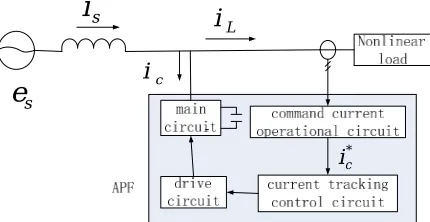
An active power filter is a new power electronic device of dynamic harmonic suppression. Figure 1 shows the basic principle. There are four parts in a shunt APF: the main circuit, command current operational circuit, cur-rent tracking control circuit, and the drive circuit. The

command current operation circuit detects the harmonic component iLh, in the load current iL, and takes the oppo-site value as command signal *

c

i . The principle can be expressed by the following formula

s L c i = +i i

L Lf Lh i =i +i

c Lh i = −i

s L c Lf i = + =i i i

where iS, iL are currents of the supply and a nonlinear load, respectively, and ic is the compensation current. iLf,

iLh are the fundamental active and harmonic reactive components of the load current, respectively.

s

i

c

i

L

i

s

e

* c

i

3. Adaptive Detecting Algorithm

3.1 The Basic Principle of Adaptive Interference Canceling Theory

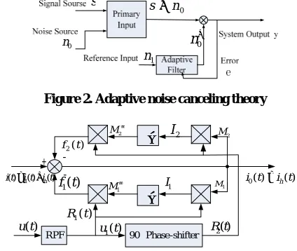
The adaptive interference canceling technique has been widely used in recent years [6]. By continuously self- studying and self-adjusting, the detecting system can always operate at its best. The basic noise-canceling the-ory can be illustrated in Figure 2. In the detecting system, there are two unrelated input signals: original input s+n0 and reference input n1. And s is unrelated with n0 and n1, while n0 and n1 are related. The reference input signal n1 is filtered by an adaptive filter to produce an output sig-nal *

0

n , which is an approximate replica of n0. This

output n*0 is subtracted from the original input signal

s+n0 to produce

* 0 0

y= + −s n n , the system output sig-nal.

In the system shown in Figure 2, the reference input is processed by an adaptive filter which automatically ad-justs its own response through a least-squares algorithm. Thus the filter can detect the noise n0 continuously and adjust the system to minimize the error signal e. It can be proved that *

0

n is the best least-squares estimate of n0, when the filter is adjusted to make the error signal power

2

[ ]

Eε minimum.

3.2 Adaptive Harmonic Detection

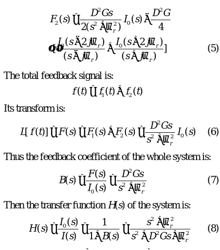
Based on the principle of adaptive noise canceling theory, adaptive harmonic current detecting circuit is shown in Figure 3. The system is composed of an analog adaptive filter, a BPF (Band Pass Filter) and a 900 phase-shifter [7]. The primary input is the load current:

1

( ) ( ) _h( ) _p( ) _q( ) _h( )

i t =i t +i t =i t +i t +i t , where i1(t) is the fundamental current, ih(t) is the sum of all harmonic components, and ip(t), iq(t) are the active component and the reactive component of i1(t), respectively in Figure 3.

u(t) and u1(t) are the AC source voltage and its funda-mental component, respectively. R1(t) and R2(t) are two reference inputs orthogonal to each other, and i0(t) is the system output.

As shown in Figure 3, because both feedback branches are similar, we take the lower feedback branch as an example. Only the fundamental reactive component which has the same frequency with R t1( ) can produce

the DC signal after the output current i0(t) is multiplied by R t1( )=Dcosωrt, while other components produce

AC signals after the same procession. The DC compo-nent can be integrated to get the average value of funda-mental reactive current IFp, while the AC component will be zero after the same calculation. Thus, we can get the instantaneous fundamental reactive current ifq(t) by

0 n 1 n s 0 n s + ∗ 0 n

Figure 2. Adaptive noise canceling theory

∫

∫

90° Phase-shifter

1( )

u t R2(t)

) ( 1 t R RPF 1 M 2 M 1 M′ 2 M′ 1 I 2 I

1( )

f t ) ( 2 t f ) ( ) (

0t i t

i = h

) ( ) ( ) (t i1t it

i = +h

+

-) (t u

Figure 3. Adaptive detecting diagram for harmonic curre- nts

multiply IFp with R1(t). Similarly, using R2(t), we can get the instantaneous fundamental active current ifp(t). At last, by adding the reverse of ifp(t)+ifq(t) to i(t), the output current i0(t)=ih(t) is produced. If only the current

i0(t)=ih(t)+ifq(t) is needed, what we should do is remove the R1(t) branch.

We can also explain the principle in the phase space. Assume the reference inputs which processed by the BPF are:

1( ) cos r R t =D ωt,

2( ) sin r R t =D ωt.

Then the output of the multiplier M1 can be expressed as:

0( ) 1( ) 0( ) cos 0( )

2

r D i t ⋅R t =i t ⋅D ωt= i t

[exp(jωrt) exp( jωrt)]

× + − (1)

Taking the Laplace transform of (1), we have

0 1 0 0

[ ( ) ( )] ( ) ( )

2 r 2 r

D D

L i t ⋅R t = I s− jω + I s+ jω (2)

where, I0(s) is the Laplace transform of i0(t). After

proc-essed by the integrator, whose transform is G

s (here G

is the integration gain), the transform of the feedback signal can be expressed as:

1( ) [ (0 ) 0( )]

2 r r

DG

W s I s j I s j

s ω ω

= − + + (3)

The output of the multiplier ' 1

M is simply the

feed-back signal of the lower branch, which mean

1( ) 1( ) 1( )

1( ) [ 1( ) 1( )]

2 r r

D

F s = W s− jω +W s+ jω

2

0 0

[ ( 2 ) ( )]

4( r) r

D G

I s j I s

s jω ω

= − +

−

2

0 0

[ ( 2 ) ( )]

4( r) r

D G

I s j I s

s jω ω

+ + +

−

2

2 2

0 2 ( )

4

2( r)

D Gs D G

I s

s ω

= +

+ (4)

Similarly, the transform F2(s) of the feedback signal

f2(t) for the upper feedback branch can be expressed as:

2 2

2( ) 2 2 0( )

4

2( r)

D Gs D G

F s I s

s ω

= −

+

0( 2 ) 0( 2 )

[ ]

( ) ( )

r r

r r

I s j I s j

s j s j

ω ω

ω ω

− +

× +

− + (5)

The total feedback signal is:

1 2

( ) ( ) ( )

f t = f t + f t

Its transform is:

2

1 2 2 2 0

[ ( )] ( ) ( ) ( ) ( )

r D Gs

L f t F s F s F s I s

s ω

= = + =

+ (6)

Thus the feedback coefficient of the whole system is:

2 2 2 0

( ) ( )

( ) r

F s D Gs

B s

I s s ω

= =

+ (7)

Then the transfer function H(s) of the system is:

2 2 0

2 2 2

( ) 1

( )

( ) 1 ( )

r

r

I s s

H s

I s B s s D Gs

ω ω

+

= = =

+ + + (8)

From (8), when ω ω= r, |H j( ω) | 0= , which means

a zero point exists in the system corresponding to the fundamental frequency ωr Consequently the funda-

metal signal will be greatly attenuated. It is obvious that the system shown in Figure 3 is equivalent to an ideal second-order notch filter. In addition, the center fre-quency of the system depends solely on the frefre-quency signal ωr of the reference input. Therefore, the system

is independent of parameter of the circuit components, which means that the system is almost stable while the temperature varies or the circuit components ages.

3.3 DC Side Voltage Control

Ideally, what an active filter compensates is the non-active power; that is to say, it neither absorbs active power from the power supply nor outputs to it, so the DC side voltage of an active filter is constant. However, due to the loss of the active filter, energy in the capacitoron

t

r

ω sin

i

p

i

∆

Figure 4. DC voltage control block diagram

the DC side will reduce, making the voltage on the ca-pacitor drop.

In order to maintain the voltage on the capacitor, the feedback method has usually been adopted, whose pur-pose is to obtain some active power from the source to compensate the corresponding loss.

As shown in Figure 4, Ucr , Ucf are the reference and feedback values of Uc, respectively. The difference be-tween Ucr and Ucf is regulated by PI to get the signal

p i

∆ .

Since ic* contains the fundamental active component ,

ic, which comes from i*c, also contains such a compo-

nent. Therefore, when ic is introduced into the power system, APF can exchange the active energy between AC and DC sides, which keeps Uc constant.

4. Simulation Results

In this section, computer simulation is carried out to ver-ify the design of the adaptive shunt active filter. A three-phase distribution system is built using Matlab as shown in Figure 5. Simulation parameters are as follow-ing: AC source is 220V/50Hz, supply side inductance Ls

is 0.2μH. The nonlinear load parameters for three-phase full-controlled bridge rectifier are R= 20Ω, L=0.1H. In themain circuit of theactive filter, IGBT is used as the switch, and the inductance on the AC side La is 5mH, while the capacitance is 2200μF/1000V on the DC side.

Figure 6 shows the AC source voltage, the power sup-ply currents before and after filterd, respectively, and the harmonic and reactive reference currents. From Figure 6(b), we can see that before filtered, the current lags the source voltage and contains a lot of harmonic and reac-tive components. After filtered by the APF, shown in Figure 6(d), the supply current is nearly sinusoidal and in phase with AC source voltage, which means APF cor-rects the power factor of the supply side nearly to unity. There is a variation in the nonlinear current at t=0.1s, From Figure 6 it can be seen the proposed adaptive shunt active filter only needs approximately half a cycle to adapt itself to the change.

Since the APF adopts traditional hysteresis current control method, the tracking ability of APF is limited, resulting in some ripples in the current when it changes suddenly, as shown in Figure 6(d).

Figure 5. Active filter simulation model

Figure 6. Simulation result of detection for harmonic and reactive currents. (a) ac source voltage for phase A, (b) power sup-ply currents for phase A before filter input, (c) harmonic and reactive reference current from adaptive detection, (d) power supply currents for phase A after filter input

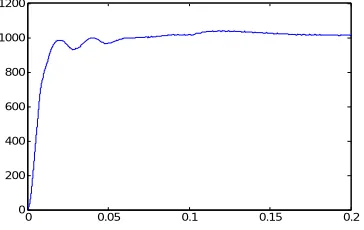
0 0.05 0.1 0.15 0.2

0 200 400 600 800 1000 1200

Figure 7. DC side capacitor voltage of active filter

Figure 9. FFT analysis of the supply current after APF in-put based on adaptive interference canceling theory

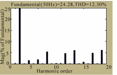
Figure 10. FFT analysis of the supply current after APF input based on instantaneous inactive power theory

takes about 0.05s to reach at the desired value of 1000V and stabilize rapidly.

Compared Figure 8 with Figure 9, it shows the har-monic and reactive currents are greatly restrained.

It shows from Figure 9 and Figure 10, under the same conditions, after APF input, the THD of the supply cur-rent based on adaptive interference canceling theory drops to 10.50%, but that based on instantaneous inactive power theory is only 12.30%, moreover, the method based on traditional theory uses 6 analog summer, 4 mul-tipliers and lots of gains, thus the calculation accuracy is more difficult to be assured in practice. The method based on adaptive interference canceling theory uses only 6 multipliers and 3 integrators, which ensures better per-formance in actual operation than that based on instanta-neous inactive power theory.

Overall, it shows that the proposed adaptive shunt ac-tive filter can compensate nonlinear load current, adapt itself to compensate the variations in nonlinear load cur-rents and correct the power factor of the supply side nearly to unity.

5. Conclusions

In this paper, a novel adaptive detection method for har-monic and reactive current is proposed. This method is analyzed systematically and verified by Matlab simula-tion. It is a continuously regulated closed-loop system,

and the operating characteristics are nearly independent of the parameter variations of the elements, and band-width behaving as one of a second-order notch filter can be regulated easily by controlling the amplitude of the reference input and the gain of the integrator. Further-more, this paper also introduces DC side voltage control method, which is simple and effective. Finally, simu-lation result is given to conform the feasibility of the design.

REFERENCES

[1] R. Bojoi, G. Griva, F. Profumo, M. Cesano, and L. Natale, “Shunt active filter implementation for induc-tion heating applicainduc-tions,” Applied Power Electronics Conference and Exposion, Vol. 3, pp. 1674–1679, March 2005.

[2] D. Liu, B. D. Zhang, and X. L. Zhang, “Design of adaptive increment controlled hybrid-type active power filter,” Power and Energy Engineering Conference, Asia-Pacific, Vol. 27–31, No. 3, pp. 1–4. 2009.

[3] H. Akagi, E. H. Watanabe, and M. Aredes, “ Instanta-neous power theory and applications to power condi-tioning,” Wiley-Interscience a John Wiley & Sons, Inc., Publication, 2007.

[4] H. Akagi, “Generalized theory of instantaneous reac-tive power and its application,” Elec.Eng. in Japanese, April 1983.

[5] L. H. Tey and Y. C. Chu, “Improvement of power quality using adaptive shunt active filter,” IEEE Transactions on Power Delivery, Vol. 20, pp. 1558–1568, April 2005.

[6] B. Widrow and S. P. Sterns, “Adaptive signal proc-essing,” Englewood Cliffs, Prentice-Hall, NJ, inc., 1985.

[7] J. H. Husy and M. S. E. Abadi, “Unified approach to adaptive filters and their performance,” IET Signal Proc-ess, Vol. 2, No. 2, pp. 97–109, 2008.

[8] A. Nakajima, “Development of active filter with se-ries resonant circuit,” IEEE-PESC, Annual Meeting, pp. 1168–1173, 1988.

[9] Q. Wang, N. Wu, and Z. A. Wang, “A neuron adap-tive detecting approach of harmonic current for apf and its realization of analog circuit,” IEEE Transac-tions on instrumentation and measurement,” Vol. 50, pp. 77–84, February 2001.

[10] H. P. To, F. Rahman, and C. Grantham, “An adaptive algorithm for controlling reactive power compensa-tion in active power filters,” Industry Applications Conference, 39th IAS Annual Meeting, Vol. 1, pp. 3– 7, October 2004.