Galaxy and Mass Assembly (GAMA) : maximum likelihood determination of the luminosity function and its evolution

Galaxy and Mass Assembly (GAMA): maximum-likelihood determination

of the luminosity function and its evolution

J. Loveday,

P. Norberg,

I. K. Baldry,

J. Bland-Hawthorn,

S. Brough,

M. J. I. Brown,

S. P. Driver,

L. S. Kelvin

and S. Phillipps

2_{Institute for Computational Cosmology, Department of Physics, Durham University, South Road, Durham DH1 3LE, UK}

3_{Astrophysics Research Institute, Liverpool John Moores University, IC2, Liverpool Science Park, 146 Brownlow Hill, Liverpool L3 5RF, UK} 4_{Sydney Institute for Astronomy, School of Physics, University of Sydney, NSW 2006, Australia}

5_{Australian Astronomical Observatory, PO Box 915, North Ryde, NSW 1670, Australia} 6_{School of Physics, Monash University, Clayton, Victoria 3800, Australia}

7_{International Centre for Radio Astronomy Research (ICRAR), The University of Western Australia, 35 Stirling Highway, Crawley WA6009, Australia} 8_{School of Physics & Astronomy, University of St Andrews, North Haugh, St Andrews KY16 9SS, UK}

9_{Institut f¨ur Astro-und Teilchenphysik, Universit¨at Innsbruck, Technikerstraße 25, A-6020 Innsbruck, Austria} 10_{Astrophysics Group, HH Wills Physics Laboratory, University of Bristol, Tyndall Avenue, Bristol BS8 1TL, UK}

Accepted 2015 May 3. Received 2015 April 29; in original form 2015 February 21

A B S T R A C T

We describe modifications to the joint stepwise maximum-likelihood method of Cole in order to simultaneously fit the Galaxy and Mass Assembly II galaxy luminosity function (LF), corrected for radial density variations, and its evolution with redshift. The whole sample is reasonably well fitted with luminosity (Qe) and density (Pe) evolution parametersQe,Pe≈1.0,

1.0 but with significant degeneracies characterized byQe≈1.4−0.4Pe. Blue galaxies exhibit

larger luminosity density evolution than red galaxies, as expected. We present the evolution-corrected r-band LF for the whole sample and for blue and red subsamples, using both Petrosian and S´ersic magnitudes. Petrosian magnitudes miss a substantial fraction of the flux of de Vaucouleurs profile galaxies: the S´ersic LF is substantially higher than the Petrosian LF at the bright end.

Key words: galaxies: evolution – galaxies: luminosity function, mass function – galaxies: statistics.

1 I N T R O D U C T I O N

The luminosity function (LF) is perhaps the most fundamental model-independent quantity that can be measured from a galaxy redshift survey. Reproducing the observed LF is the first require-ment of a successful model of galaxy formation, and thus accurate measurements of the LF are important in constraining the physics of galaxy formation and evolution (e.g. Benson et al.2003). In addi-tion, accurate knowledge of the survey selection function (and hence LF) is required in order to determine the clustering of a flux-limited sample of galaxies (Cole2011).

A standard 1/Vmax(Schmidt1968) estimate of the LF is

vulnera-ble to radial density variations within the sample. This vulnerability can be largely mitigated by multiplying the maximum volume in which each galaxy is visible,Vmax, by the integrated radial

over-density of a over-density-defining population (Baldry et al.2006,2012). Maximum-likelihood methods (Sandage, Tammann & Yahil1979;

_{E-mail:J.Loveday@sussex.ac.uk}

Efstathiou, Ellis & Peterson1988), which assume that the lumi-nosity and spatial dependence of the galaxy number density are separable, are, by construction, insensitive to density fluctuations. However, if the sample covers a significant redshift range, galaxy properties (such as luminosity) and number density are subject to systematic evolution with lookback time. All of the above methods must then either be applied to restricted redshift subsets of the data, or be modified to explicitly allow for evolution (e.g. Lin et al.1999; Loveday et al.2012).

Cole (2011) recently introduced a joint stepwise maximum-likelihood(JSWML) method, which jointly fits non-parametric es-timates of the LF and the galaxy overdensity in radial bins, along with an evolution model. In this paper, we describe modifications made to the JSWML method in order to successfully apply it to the Galaxy and Mass Assembly (GAMA) survey (Driver et al.

2011). In the GAMA-II sample,L∗galaxies can be seen out to red-shiftz≈0.35, and so one has a reasonable redshift baseline over which to constrain luminosity and density evolution. Loveday et al. (2012) have previously investigated LF evolution in the GAMA-I sample, finding that at higher redshifts: all galaxy types were more

C

luminous, blue galaxies had a higher comoving number density and red galaxies had a lower comoving number density. Here, we exploit the greater depth (0.4 mag) of GAMA-II versus GAMA-I, and use an estimator of galaxy evolution that does not assume a parametric form (e.g. a Schechter function) for the LF.

The paper is organized as follows. In Section 2, we describe the GAMA data used along with corrections made for its small level of incompleteness. Our adopted evolution model is described in Section 3 and the density-correctedVmaxmethod in Section 4.

Methods for determining the evolution parameters are discussed in Section 5. We present tests of our methods using simulated data in Section 6 and apply them to GAMA data in Section 7. We briefly discuss our findings in Section 8 and conclude in Section 9.

Throughout, we assume a Hubble constant of H0 =

100hkm s−1_Mpc−1_{and an}

M=0.3, =0.7 cosmology in

cal-culating distances, comoving volumes and luminosities.

2 G A M A - I I DATA , K- A N D C O M P L E T E N E S S C O R R E C T I O N S

In 2013 April, the GAMA survey completed spectroscopic coverage of the three equatorial fields G09, G12 and G15. In GAMA-II, these fields were extended in area to cover 12◦ ×5◦each1 _and

all galaxies were targeted to a Galactic-extinction-corrected Sloan Digital Sky Survey (SDSS; Abazajian et al.2009) DR7 Petrosianr -band magnitude limit ofr=19.8 mag. In our analysis, we include all main-survey targets (SURVEY_CLASS≥4)2_{with reliableAUTOZ}

(Baldry et al.2014) redshifts (nQ≥3) from TilingCatv43 (Baldry et al.2010). Redshifts (from DistancesFramesv12) are corrected for local flow using the Tonry et al. (2000) attractor model as described by Baldry et al. (2012).

We calculate LFs using both Petrosian (1976) and S´ersic (1963) photometry, corrected for Galactic extinction using the dust maps of Schlegel, Finkbeiner & Davis (1998). We use single S´ersic model magnitudes truncated at 10 effective radii as fit by Kelvin et al. (2012). Kelvin et al. (2012) show that these recover essentially all of the flux for ann=1 (exponential) profile, and about 96 per cent of the flux of ann=4 (de Vaucouleurs) profile. SDSS Petrosian magnitudes, while also measuring almost all of the flux for expo-nential profiles, measure only about 82 per cent of the flux for de Vaucouleurs profiles (Blanton et al.2001). S´ersic magnitudes are, however, more susceptible to contamination from nearby bright ob-jects, which can cause them to be overestimated by several mag. We identify galaxies that may have contaminated photometry by searching for brighter stellar neighbours within a distance, up to a maximum of 5 arcmin, of twice the star’s isophotal radius (isoA_r in the SDSSPhotoObjtable). Five per cent of GAMA targets are flagged in this way.

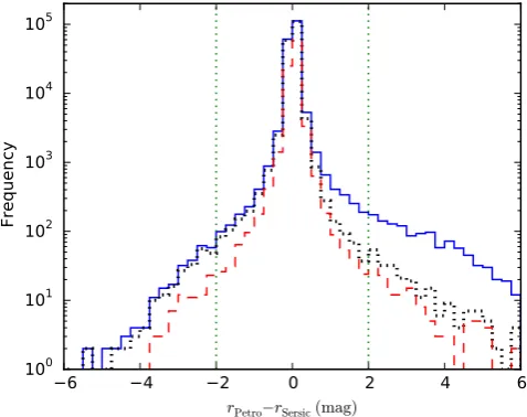
Fig. 1 shows a histogram of m = rPetro − rSersic for all

GAMA-II main-survey targets (continuous blue histogram), and for targets without a nearby bright stellar neighbour (black dotted histogram). The majority (about 72 per cent) of excluded galaxies have positivem, i.e. are brighter in S´ersic than Petrosian magni-tude. The dashed red histogram indicates targets without a nearby

1_{The RA, Dec. ranges of the three fields, all in degrees, are G09: 129.0–}

141.0,−2.0 to+3.0; G12: 174.0–186.0,−3.0 to+2.0; G15: 211.5–223.5,

−2.0 to+3.0.

2_{Note that in this latest version of TilingCat, objects that failed visual}

inspection (VIS_CLASS=2, 3 or 4) also have SURVEY_CLASS set to zero.

Figure 1. Histogram of the difference between Petrosian and S´ersic mag-nitudes for all GAMA-II main-survey targets (continuous blue histogram), and for targets without a nearby bright stellar neighbour, as defined in the text (black dotted histogram). The dashed red histogram indicates the subset of the latter targets classified as red. The vertical dotted lines denote the additional constraint|rPetro−rSersic|<2.0 mag required for galaxies to be

assumed uncontaminated; only about 0.3 per cent of remaining targets lie beyond these limits.

bright stellar neighbour that are classified as red (as defined towards the end of this section). It is clear from this figure that uncontami-nated red galaxies preferentially have brighter S´ersic than Petrosian magnitudes. This is as expected, assuming that they are bulge dom-inated, and hence have profiles with higher S´ersic index.

We exclude an additional 487 targets (0.3 per cent of the total) for which ther-band S´ersic and Petrosian magnitudes differ by more than 2 mag. This magnitude difference cut is somewhat arbitrary, but is designed to exclude galaxies with bright stellar neighbours that do not quite satisfy the above criterion (for instance if a galaxy lies on a star’s diffraction spike) or with bad sky background determination. It seems extremely unlikely that the S´ersic magnitude would recover more flux than this from an uncontaminated galaxy.

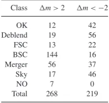
We have visually inspected these additional culled targets, for which|m| = |rPetro−rSersic|>2 mag, and placed them in one of

Table 1. Classification of the 487 GAMA targets without a bright stellar neighbour (as de-fined in the text) for which

m=rPetro−rSersiclies outside

the range [−2, 2] mag. See text for meaning of first column.

Class m>2 m<−2

OK 12 42

Deblend 19 56

FSC 13 22

BSC 144 16

Merger 56 37

Sky 17 46

NO 7 0

Total 268 219

are expected to be more luminous than average. In cases when the Petrosian and S´ersic magnitudes differ by more than 2 mag, both magnitude estimates are suspect, and so it is debatable whether these objects should be GAMA targets at all. At worst, the effect of excluding targets with bright stellar neighbours or discrepant magnitudes (5.3 per cent of the entire GAMA-II sample) will be to bias the LF normalization low by up to 5 per cent.

After excluding GAMA main-survey targets with either an unre-liable redshift (1.2 per cent) or suspect photometry (5.3 per cent), we are left with a sample of 173 527 galaxies in the redshift range 0.002< z <0.65.

To determineK-corrections, we useKCORRECTv4.2 (Blanton &

Roweis2007) to fit spectral energy distributions tougrizGAMA matched-apertureSEXTRACTOR(Bertin & Arnouts1996)AUTO

magni-tudes taken from ApMatchedCatv04 (Hill et al.2011). As shown in appendix B of Taylor et al. (2011) and fig. 17 of Kelvin et al. (2012), SDSS model magnitudes, which have been recommended for cal-culating galaxy colours, e.g. Stoughton et al. (2002), are ill-behaved for galaxies of intermediate S´ersic index which are well fitted by neither pure exponential nor pure de Vaucouleurs profiles. GAMA matched-aperture magnitudes do not force a particular functional form on the galaxy profile and so provide more reliable colours for all galaxy types. In practice, we find that the choice of magnitude type used forK-corrections makes little difference to our LF esti-mates, with the Schechter fit parameters changing by less than 1σ. We useK-corrections to reference redshiftz0=0.1 in order to

al-low direct comparison with previous results (Loveday et al.2012). For the three GAMA-II targets that are missingAUTOmagnitudes,

and for the 3.3 per cent of targets for whichKCORRECTreports aχ2

statistic of 10.0 or larger, implying a poor spectral energy distribu-tion (SED) fit, we set theK-correction to the mean of the remaining sample. We have visually inspected 235 of these targets with poor-fitting SEDs. About 29 per cent are close to a bright star or are otherwise likely to suffer from poorly estimated sky background; about 22 per cent have one or more close neighbours and may thus suffer contaminated photometry; about 13 per cent show evidence of AGN activity. The remaining 35 per cent show no obvious reason for the SED fit to be poor, but it seems likely that many of these cases may be due to pooru-band photometry with underestimated errors.

While SDSS DR7 has improved photometric calibration over DR6 (used for selection of GAMA-I targets), it will suffer from the same surface-brightness-dependent selection effects as DR6, and so we assume the sameimaging completeness Cimas shown in fig. 1

Figure 2. Redshift success rate as a function ofr-band fibre magnitude. The top panel shows histograms ofrfibrefor all observed galaxies in blue, and

galaxies with a reliable redshift measurement (nQ>2) in green. Redshift success, the ratio of the latter to the former, is shown as a histogram in the lower panel, along with a best-fitting sigmoid-type function. The large fluctuations at faint magnitudes (rfibre>21) are simply due to small-number

statistics: the success rate is the ratio of two small numbers.

of Loveday et al. (2012). In this paper, we only measure ther-band LF, and so assume thattarget completenessis 100 per cent. In fact, just 0.1 per cent of GAMA-II main targets withr<19.8 mag lack a measured spectrum, with no systematic dependence on magnitude (Liske et al., submitted to MNRAS). Since GAMA-II uses a new, fully automated redshift measurement (Baldry et al.2014), we have re-assessedredshift success ratefor GAMA-II. Fig.2shows red-shift success rate, defined as the fraction of observed galaxies with reliable (nQ≥3) redshifts, as a function ofr-band fibre magnitude. This success rate is well fitted by a modified sigmoid function

Cz=[1+ea(rfibre−b)]−c (1)

with parametersa=2.55 mag−1_{,b=22.42 mag and c= 2.24.}

The extra parameterc(cf. Ellis & Bland-Hawthorn2007; Loveday et al.2012) is introduced to provide a more extended decline inCz

aroundrfibre≈20 mag. Without it, the sigmoid function drops too

sharply to faithfully follow the observedCz.

Each galaxy is given a weight equal to the reciprocal of the product of imaging completeness and redshift success rate,

Wi=1/(CimiCzi). A histogram of these weights is shown in Fig.3. While the vast majority of galaxies (99.5 per cent) haveWi<2, there is a tail of rare objects with weights as high as 100 or more. We have visually inspected the 157 objects with an assigned weight above 10.0. Of these, 38 per cent are close to a bright star or are oth-erwise likely to have a poorly determined sky background; another 38 per cent have nearby neighbouring galaxies, which might lead to a compromised surface-brightness estimate; 10 per cent are iso-lated and show no obvious visual indication of being of low surface brightness. That left just 14 per cent that appeared to be genuine low brightness galaxies, potentially with half-light surface-brightness μ50,r24 mag arcsec−2and/or with fibre magnitude

rfibre22 mag. We therefore chose to set an upper limit cap of 5.0

Figure 3. Histogram of completeness-correction weights for GAMA-II galaxies. Note that both axes use logarithmic binning. The vertical line corresponds to the applied upper limit weight cap of 5.0.

corresponds to the inverse redshift success rate for galaxies with the faintest fibre magnitudes (Fig.2). While only 297 galaxies (0.16 per cent of the total) haveWi>5.0, these galaxies are likely to lie at the extreme faint end of the LF, where there are few observed galaxies, and so spurious weights could potentially bias the LF faint end. The mean galaxy weights before and after applying this cap are 1.12 and 1.09, respectively.

The effect of applying this weight cap is to reduce the best-fitting value of the density evolution parameterPeby about 40 per cent,

with a corresponding increase in the best-fitting value of the lumi-nosity evolution parameterQe. Best-fitting LF parameters change

by less than 1σ.

When subdividing GAMA galaxies into blue and red subsamples, we use the colour cut of Loveday et al. (2012), namely

0.1

(g−r)Kron=0.15−0.030.1(Mr−5 logh). (2)

A detailed investigation of colour bimodality in GAMA has recently been presented by Taylor et al. (2015). They utilize restframe and dust-corrected (g−i) colour, and argue that a probabilistic assign-ment of galaxies to ‘R’ and ‘B’ populations is preferable to a hard (and somewhat arbitrary) red/blue cut. They also emphasize that colour is not synonymous with morphological type, but rather pro-vides a proxy for mean stellar age within a galaxy. Also, of course, a galaxy may appear red in uncorrected restframe colour due to dust extinction, rather than an old stellar population. In this paper, we stick with the simple colour cut of equation (2) for two reasons: (i) to allow direct comparison with the results of Loveday et al. (2012) and (ii) the Taylor et al. (2015) model of the colour–mass distribution has been tuned to a nearly volume-limited sample of galaxies at redshiftz <0.12 – the model parameters are likely to evolve at higher redshift.

Uncertainties in measured quantities, such as radial overdensity and the LF, are determined by jackknife resampling. We subdivide the GAMA-II area into nine 4◦×5◦regions, and then recalculate the quantity nine times, omitting each region in turn. For any quantity

x, we may then determine its variance using

Var(x)= N−1

N

N

i=1

(xi−x¯)2, (3)

whereN=9 is the number of jackknife regions,xiis our estimate ofxobtained when omitting regioniand ¯xis the mean of thexi. The numerator (N− 1) in the pre-factor allows for the fact that the jackknife estimates are not independent. Each jackknife region

contains an average of 19 281 galaxies for the full GAMA-II sample (i.e. without colour selection).

3 PA R A M E T R I Z I N G T H E E VO L U T I O N

We parametrize luminosity and density evolution over the redshift range 0.002< z <0.65 using the parametersQeandPeintroduced

by Lin et al. (1999). This model assumes that galaxy populations evolve linearly with redshift in absolute magnitude, parametrized byQe, and in log number density, parametrized byPe. Specifically,

the luminositye-correction is given byE(z)=Qe(z−z0), such that

absolute magnitudeMis determined from apparent magnitudem

using

M=m−5 log10dL(z)−25−K(z;z0)+Qe(z−z0), (4)

wheredL(z) is the luminosity distance (assuming the

cosmolog-ical parameters specified in the Introduction) at redshift z and

K(z;z0) is theK-correction, relative to a passband blueshifted by

z0. Luminosity evolution is determined relative to the same redshift

z0=0.1 as theK-correction.

Evolution in number densityP(z) is parametrized as

P(z)=P(z0)100.4Pe(z−z0)=P(z=0)100.4Pez. (5)

The motivation for this choice of parametrization is that if the shape of the LF does not evolve with redshift, that is it shifts only horizontally in absolute magnitude byQe, and vertically in

log-density byPe, then luminosity densityρLevolves as

ρL(z)=ρL(z0)100.4(Pe+Qe)(z−z0). (6)

WhilePeandQeare strongly degenerate, and so poorly constrained

individually, their sum Pe + Qe is well constrained (Lin et al.

1999; Loveday et al.2012). We set further constraints on the linear combination of these parameters in Section 7.

4 D E N S I T Y- C O R R E C T E D Vmax M E T H O D

In this section, we describe our technique for determining the LF using a maximum-likelihood, density-correctedVmaxestimator,

as-suming that evolution is known. We will discuss how we determine the evolution parametersQe and Pe in Section 5. Our method is

based on the JSWML method of Cole (2011), which jointly fits the LF and overdensities in radial bins of redshift caused by large-scale structure. Cole’s derivation starts with an expression for the

jointprobability of finding a galaxy at specified redshift and lumi-nosity, and assumes that all galaxies have identical evolution- and

K-corrections. We wish to allow for individualK- (and in the future

e-) corrections, in which case it is easier to start with theconditional

probability that an observed galaxy of luminosityLihas a redshiftzi, assuming that the luminosity and spatial dependence of the galaxy number density are separable. This conditional probability is given by (Saunders et al.1990):

pi=

(zi)P(zi) d_dV_zz i zmax,i

0 (z)P(z) dV dzdz

. (7)

Here, we have factored the mean density at redshift z, ¯n(z)=

(z)P(z), into a product of the galaxy overdensity3_{(z) due to}

large-scale structure times the steadily evolving densityP(z) from

3_{Following Cole (2011), we use the term overdensity to mean a}

equation (5);dV/dzis the differential of the survey volume, and

zmax,i is the maximum redshift at which galaxyiwould still be visible, determined by the survey flux limit along with the galaxy’s luminosity,K- ande-corrections.

Adopting binned estimates of the galaxy overdensity, and weighting each galaxy by its incompleteness-correction weight,Wi, we obtain a log-likelihood

lnL=

i

Wi ⎡

⎣ln

j

jPjVjDij −ln

j

jPjVjSij ⎤

⎦. (8)

HereVj,Pjandjare the volume, density evolution and galaxy overdensity, respectively, in redshift bin j; the function Dij is a simple binning function, equal to unity if galaxyilies in redshift binj, zero otherwise, andSijis the fraction of redshift binjin which galaxyiis visible. In the present analysis, we employ redshift bins of width z = 0.01. The maximum-likelihood solution for the overdensitiesj, given by ∂lnL/∂j=0, may be obtained by

iteration from:

j =Wsum,j

i

WiPjVjSij

Vdc maxi

−1

, (9)

whereWsum,j=

iWiDijis the sum of galaxy weights in redshift binjandVdc

maxi=

kkPkVkSik, the effective volume, corrected

for evolution and fluctuations in radial density, within which galaxy

iis visible.

The LF, unaffected by density fluctuations, may then be estimated by substitutingVdc

maxfor the usual expression forVmax:

φbin

l =

i

WiDil

Vdc maxi

, (10)

whereDil=1 if galaxyiis in luminosity binl, zero otherwise. Cole (2011) shows that this expression may be derived via maximum likelihood, at least in the case of identicale- andK-corrections.

Cole also discusses an extension to this method whereby pa-rameter(s) describing the density evolutionP(z) may be determined simultaneously with the overdensitiesjby adding prior constraints on the values ofjusing the known clustering of galaxies. However, for our choice of density evolution parametrization (equation 5), the derivative in Cole equation (25) no longer depends explicitly on the evolution parameter, leading to a lack of convergence. We there-fore prefer to search over both luminosity and density evolution parameters, as described in the next section.

A stepwise estimate of the LF, as given by equation (10), is not constrained to vary smoothly from bin to bin. Furthermore, at very low and high luminosity there may be bins containing no galaxies, resulting in an ill-defined log-likelihood (see equation 12 below). This problem is exacerbated when exploring possible values of the luminosity evolution parameterQe, as galaxies will then shift from

bin to bin asQe is varied, resulting in unphysical sharp jumps in

likelihood. To overcome these problems, we employ a Gaussian-smoothed estimate of the LF:

φlGS= i Wi Vdc maxi G

Mi−Ml

b

. (11)

Here, the smoothing kernel G is a standard Gaussian, b is the smoothing bandwidth,Miis the (K- ande-corrected) absolute mag-nitude of galaxyiandMlis the absolute magnitude at the centre of binl. In order not to underestimate the extreme faint end of the LF, it is important to apply boundary conditions toφGS_{corresponding}

to the chosen range of absolute magnitudes. We do this using the

default renormalization method and bandwidth choice of the python modulepyqt_fit.kde.4φGSdoes not, of course, correspond to the

true galaxy LF, but rather to the LF convolved with a Gaussian of standard deviationb. Therefore, when plotting the LF and fitting a Schechter function, we use the standard binned LFφbin_rather

thanφGS_.

5 D E T E R M I N I N G E VO L U T I O N PA R A M E T E R S

In Cole’s original derivation of this method, one maximizes a pos-terior likelihood (Cole equation 38)5_{over the luminosity evolution}

parameterQe (Cole calls this parameter u). When applying this

method to GAMA data, we found that the estimated value ofQe

diverged, unless one places an extremely tight prior on its value.6

Our problem was traced to the fact that varyingQechanges all of the

inferred absolute magnitudes (as well as visibility limits) for each galaxy. Choosing fixed absolute magnitude limits within which to determine the LF thus results in a change of sample size asQevaries,

leading to likelihoods that cannot be directly compared. Even if one includes the term on the second line of Cole equation (36), which yields−Ntotln ˆNtotin the case of identicalK- ande-corrections, the

estimate ofQestill diverges as galaxies shift systematically brighter

or fainter asQedecreases or increases. We therefore consider two

alternative methods to optimize the evolution parameters.

5.1 Mean probability

Our first solution is to consider not the product of the probabilities of observing each galaxy, but instead thegeometric meanof the probabilities, which does not vary systematically with sample size

N. Our pseudo-log-likelihood lnPis then given by (Cole equation 36)

lnP= 1

N

j

Wsum,jln(VjPjj)+

1

N

l

Wsum,llnφlGS

−1

N

i

Wiln

j

VjPjj

l

φGS_l S(Lmin,i,j|Ll)

−

j

(j−1)2

2σ2 j

−(Qe−Q0)2

2σ2 Qe

− (Pe−P0)2

2σ2 Pe

, (12)

whereWsum,jis the sum of galaxy weights in redshift binj,Wsum,lis the sum of galaxy weights in luminosity binlandS(Lmin,i,j|Ll) is the fraction of luminosity binlfor which galaxyiat redshiftzjwould be visible. The term on the second line is a constant in the case of identicalK- ande-corrections; with identicale-corrections but independentK-corrections we find that including this term makes a negligible difference to the maximum-likelihood solution. The terms on the third line are priors on the radial overdensitiesjand

4_{https://pypi.python.org/pypi/PyQt-Fit.}

5_{Note that Cole equations (36)– (38) are missing factors ofPp, such that}

each occurrence ofVpshould readVpPp.

6_{We believe that the reason that the test described in section 5 of Cole}

the evolution parametersPeandQe. The priors onjare essential, as these values are completely degenerate with the density evolution parameterPe. As discussed by Cole, the expected variance injis given by

σ2_j =1+4πnˆjJ3

ˆ

njVj

, (13)

with ˆnj the predicted density andVjthe volume of redshift binj. The factorJ3=

r2_{ξ(r)dr≈2000h}−3_Mpc3_{accounts for the fact}

that because galaxies are clustered, they tend to come in clumps of 4πnJˆ 3galaxies at a time (Peebles1980). We find, however, that

much more reliable estimates ofσ2

j are obtained from jackknife

sampling – see Fig.6below. This is particularly true in the higher redshift bins, where one is sampling the clustering of the most lumi-nous galaxies, and where adopting a universal value forJ3

underes-timates the actual density fluctuations observed between jackknife samples. The priors onPeandQeare optional, and may help

conver-gence in some cases. We adopt broad priors of (Q0, σQ2e)=(1,1) and (P0, σP2e)=(2,1). These values were chosen to be consistent with the findings of Loveday et al. (2012) while still allowing some freedom for the optimum values to change under the present anal-ysis.

5.2 LF–redshiftχ2

Our second method compares LFs estimated in two or more red-shift ranges: if the evolution and density variations are correctly modelled, then the LFs should be in good agreement; if evolution parameters are poorly estimated, then one would expect poor agree-ment. We then minimize theχ2_{(≡ −2 lnL) given by}

χ2₌ j ,k>j

l

(φlj−φkl)2

Var(φlj)+Var(φlk)

+

j

(j−1)2

σ2 j

, (14)

whereφlj is the Gaussian-smoothed LF in magnitude binlfor the

broad redshift rangej, and Var(φj_l) is the corresponding variance, determined by jackknife resampling. We restrict the sum over mag-nitude binslto those bins which are complete given the redshift limits (see section 3.3 of Loveday et al.2012) and which include at least 10 galaxies for all values ofQebetween specified limits. In

practice, we have found best results are achieved using just two red-shift ranges, split near the median redred-shift of the sample, ¯z≈0.2, so that the ‘knee’ region of the LF aroundL∗is well-sampled by both, and hence the degeneracies between luminosity and density evolution are minimized. If one chooses three or more redshift ranges, there will be very little luminosity coverage in common to the lowest and highest ranges, and so one does not really gain much information in doing so. Again, it is essential to place a prior on the overdensities (final sum in equation 14, withσ2

j also

deter-mined from jackknife resampling) to remove the degeneracy with density evolution. This method places no priors on the values for the evolution parameters.

5.3 Finding optimum evolution parameters

We first evaluateχ2_{values, using each of the above methods, on}

a rectangular grid of (Pe,Qe), thus allowing one to visualize the

correlations between the evolution parameters. The grid point with the smallestχ2_{value is then used as a starting point for a downhill}

simplex minimization to refine the parameter values corresponding to minimumχ2_.

In order to quantify the degeneracy between evolution param-eters, we slice theχ2_{grid in bins ofP}

e. For each slice, we fit a

quadratic function toχ2_(Q

e) using the five (Qe,χ2) values closest

to the point of minimumχ2_{in that slice. Using this quadratic fit,}

we locate the pointQ_e,χ2

minof minimumχ

2_{and its 1σrange, i.e. the}

range ofQevalues whereχ2increases by unity from the minimum.

We find both for simulations and for real data that theQ_e,χ2 min–Pe re-lation is very well fitted by a straight line, and so we perform a linear least-squares fit to (Pe, Qe,χ2

min) to obtain the relationQe=mPe+c which minimizesχ2_.

6 T E S T S U S I N G S I M U L AT E D DATA

6.1 The simulations

In this section, we test our implementation of the JSWML estimator using simulated data, following the procedure outlined in section 5 of Cole (2011).

We start by choosing a model LF with Schechter (1976) and evo-lution parameters close to those obtained from the GAMA-I survey by Loveday et al. (2012) and as given in Table2. We then randomly generate redshifts with a uniform density in comoving coordinates, modulated by our assumed density evolution (equation 5), over the range 0.002 < z <0.65. Absolute magnitudes are selected ran-domly according to our assumed Schechter function from the range

−24 < M < −12. From each absolute magnitude, we subtract

Qe(z−0.1) to model luminosity evolution. We then assign

appar-ent magnitudesrusingK-correction coefficients selected randomly from the GAMA-II data and reject simulated galaxies fainter than

r=19.8. This process is repeated until sufficient random galaxies have been generated to give the required number density,

Nsim= zmax

zmin

Lmax(z,mmax)

Lmin(z,mmin)

φ(L, z)dLdV

dzdz, (15)

within a volume corresponding to that of the three GAMA-II fields, viz 3×5◦×12◦=180 deg2_.

In order to simulate the effects of galaxy clustering, we spilt the simulated volume into 65 redshift shellspof equal thickness

z≈0.01 and with volumeVj. For each shell, we generate a random density perturbation δj drawn from a Gaussian with zero mean and variance 4πJ3/Vj, with 4πJ3=30,000h−3Mpc3. We then

randomly resampleN_j =(1+δj)Nj of the originalNjsimulated galaxies in each shellp, thus producing fluctuations consistent with the assumed value ofJ3.

Imaging completeness and redshift success are modelled by gen-erating surface brightnesses and fibre magnitude for each simulated galaxy according to the relations observed in GAMA-I data, see

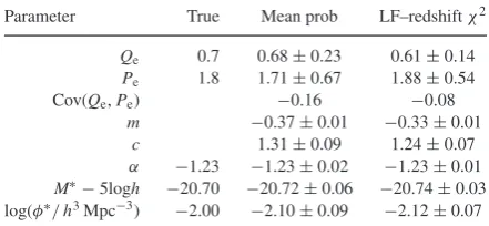
Table 2. Mean and standard deviation of the evolution and Schechter parameters recovered from 10 simulated GAMA catalogues. Param-etersmandc quantify the linear relationQe = mPe +c which

minimizesχ2.

Parameter True Mean prob LF–redshiftχ2

Qe 0.7 0.68±0.23 0.61±0.14

Pe 1.8 1.71±0.67 1.88±0.54

Cov(Qe,Pe) −0.16 −0.08

m −0.37±0.01 −0.33±0.01 c 1.31±0.09 1.24±0.07

appendix A1 of Loveday et al. (2012). Imaging completenessCim

is then determined from fig. 1 of Loveday et al. (2012) and redshift successCzfrom equation (1). Simulated galaxies are then chosen randomly with probability equal toCimCzand assigned a weight Wi=1/(CimiCzi) to compensate for those simulated galaxies omit-ted from the sample.

This procedure is repeated to generate 10 independent mock cat-alogues, each containing around 180 000 galaxies. These mock catalogues are run through the JSWML estimator, with evolution parameters being determined using both methods discussed in the previous section. Since the mock galaxies are clustered only in red-shift shells and not in projected coordinates on the sky, we determine the expected variance in overdensity using equation (13) rather than jackknife resampling. We employ 65 redshift shells out toz=0.65 and calculate the LF in bins ofM =0.25 mag over the range

−23<M<−15 mag.

6.2 Simulation results

The mean and standard deviation of each recovered parameter, and the covariance between evolution parameters, are given in Table2. We see that the input evolution and LF parameters are recovered within about one standard deviation for both methods.

Fig.4shows 95 per cent confidence limits on the evolution pa-rameters measured from each of the simulations. We see that the error contours are significantly smaller using the LF–redshiftχ2

method compared with the mean probability method. However, this

Figure 4. 95 per cent confidence limits on evolution parameters determined from 10 simulated data sets (light contours) and their average (heavy con-tour) determined using (top) mean probability (equation 12) and (bottom) LF–redshiftχ2_{(equation 14). The error bars show the mean and standard}

deviation of the (Pe,Qe) parameters from each simulation which yield

minimumχ2_{. The input evolution parameters for these simulations were}

Pe=1.8,Qe=0.7.

Figure 5. 95 per cent confidence limits on GAMA-II evolution parameters for all, blue and red galaxies as labelled. The upper panel shows the limits obtained using mean probability (equation 12); the lower panel shows results using LF–redshiftχ2(equation 14). The large dots indicate the location of minimumχ2. The large error bars show the evolution parameters and 68 per cent confidence limits estimated for the combined GAMA-I sample in ther band by Loveday et al. (2012,QparandPparfrom table 5).

test is idealized, in that our choice of evolution parametrization is identical in the simulations and in the analysis,7 _{and so we will}

apply both methods of constraining evolution parameters to the GAMA data in the following section. Note that the simulations have no inbuilt covariance between evolution parameters: they all use identical values ofPeandQe. The degeneracies (as quantified

by Cov(Qe,Pe) and the parametersmandcin Table2) arise as a

result of the fitting process. For an LF described by an unbroken power law, the degeneracy betweenPeandQewould be total, i.e.

evolution in luminosity and density would be indistinguishable.

7 R E S U LT S F R O M G A M A

7.1 Evolution

Fig.5shows 95 per cent confidence limits on the evolution param-etersPe,Qedetermined using equations (12) and (14) for the full

GAMA-II sample and for blue and red galaxies separately. We see

7_{We are performing a self-consistency test. It is unlikely that real galaxy}

Table 3. Best-fitting evolution parameters for GAMA-II galaxy samples obtained using both mean probability and LF–redshift methods. Parametersmandcquantify the linear relationQe=mPe+c. For the LF–redshift method only,χν2 is the reducedχ2_{from equation (14); The uncertainties quoted onQ}

eandPecome from

the bounding box containing the 1σlikelihood contour; the uncertainty onPe+Qe

is given by the distance from the point of minimumχ2_{to the 1σlikelihood contour}

along the directionPe=Qe.

Sample Qe Pe Qe+Pe m c χν2

Mean probability

All 1.03±0.10 1.00±0.25 2.02±0.05 −0.36 1.38 . . . Blue 1.09±0.10 1.30±0.25 2.39±0.04 −0.35 1.55 . . . Red 0.58±0.18 1.55±0.40 2.12±0.08 −0.38 1.17 . . .

LF–redshift

All 1.03±0.07 1.00±0.20 2.02±0.05 −0.35 1.37 3.76 Blue 1.18±0.05 1.07±0.15 2.25±0.04 −0.34 1.55 3.46 Red 0.73±0.10 1.25±0.25 1.98±0.06 −0.36 1.16 3.35

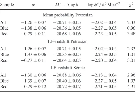
Table 4. Best-fittingr-band LF parameters for GAMA-II galaxy samples obtained using both mean probability and LF–redshift methods. For the latter method, we show LF parameters obtained using both Petrosian and S´ersic magnitudes. χ2

ν is the reducedχ2 from least-squares Schechter function fits to the LF estimates; none of the LFs is well fitted in detail by a Schechter function, particularly at the bright end. The uncertainties quoted on the LF parameters come from jackknife sampling, but do not explicitly include the large degeneracies between them.

Sample α M∗−5logh logφ∗/ h3_Mpc−3 _χ2 ν

Mean probability Petrosian

All −1.26±0.07 −20.71±0.05 −2.02±0.04 2.33 Blue −1.38±0.06 −20.36±0.05 −2.27±0.05 0.96 Red −0.79±0.11 −20.68±0.06 −2.23±0.05 3.48

LF–redshift Petrosian

All −1.26±0.07 −20.71±0.05 −2.02±0.04 2.33 Blue −1.37±0.06 −20.35±0.05 −2.24±0.05 1.01 Red −0.77±0.11 −20.64±0.05 −2.20±0.04 3.01

LF–redshift S´ersic

All −1.30±0.06 −20.88±0.06 −2.13±0.04 2.96 Blue −1.39±0.07 −20.40±0.06 −2.27±0.05 1.03 Red −0.79±0.12 −20.72±0.07 −2.21±0.05 4.91

that the confidence limits obtained with the two different methods largely overlap, although there are small differences between them. Best-fitting evolution parameters are given in Table3. The differ-ence in LFs obtained using evolution parameters determined with the two different methods is negligible (much less than the 1σ ran-dom errors; see Table4). This illustrates the robustness of the LF estimate to the individual values assumed forPeandQe: as long as

their joint estimate is reasonable, e.g. they lie within the 95 per cent likelihood contours of Fig.5, then overestimating one evolution parameter (e.g.Pe) is largely compensated for by underestimating

the other (e.g.Qe).

The differences in density evolution (Pe) for red and blue galaxies

are not significant. Blue galaxies do however exhibit significantly stronger evolution in luminosity (Qe) and in luminosity density

(Qe+Pe) than red galaxies, at the∼5σlevel.

The differences between red and blue galaxies agree qualitatively with those of Loveday et al. (2012), although in the present analysis we no longer see any evidence for negative density evolution for red galaxies. The three samples show very similar degeneracies in

(Pe,Qe) parameter space. The errors onPeandQein Table3are the

formal errors obtained by holding one parameter fixed and varying the other untilχ2 _{increases by one. Given the scatter in 95 per}

cent confidence limits between simulations shown in Fig.4, more realistic errors, and their covariance, may be obtained from Table2. Since the exact values assumed for the evolution parameters have such a small effect on the LF parameters, see Table4below, for the remainder of this paper we assume evolution parameters found from the LF–redshift method in the lower half of Table3.

7.2 Radial overdensities

Radial overdensities are shown in Fig.6. While our evolution model is performing well, insofar as(z) oscillates about unity, for red-shiftsz0.5, beyond this limit the overdensities are systematically high. This effect is almost entirely due to red galaxies, suggesting that luminosity and/or density evolution increases sharply atz≈0.5 for these galaxies compared with our model (section 3). It seems unlikely that incompleteness corrections could cause this, as there is no noticeable increase in weights beyondz=0.5. Only 0.8 per cent of GAMA-II main-survey galaxies lie beyondz=0.5, too few to constrain a more complicated evolution model, or to look for a large overdensity at these redshifts, see Fig.7.

Below redshiftsz=0.5, we see the same features in radial over-density in all three samples, although the fluctuations, as expected, are slightly more pronounced in the red galaxy sample. Note that the error bands given by equation (13) (shaded regions in Fig.6) are significantly larger/smaller than the jackknife errors at low/high redshift. There are two reasons for this: (i) the low-redshift bins sample too small a volume for theJ3integral to have converged and

(ii) the low-/high-redshift bins are dominated by faint/luminous galaxies, with weaker/stronger clustering than the average defined by the assumed value ofJ3. This is why we use jackknife errors

rather than the predicted variance in determiningσ2

δj. We have tried

halving the number of redshift bins to 32, verifying that the fitted parameters are insensitive to the redshift binning, with parameters changing by less than 1σwhen the redshift bin size is doubled from

z=0.01 toz=0.02.

7.3 LFs

Figure 6. Radial overdensities determined from GAMA-II using the entire sample and blue and red subsets as labelled, assuming evolution parameters as given in the lower half of Table3. The error bars show uncertainties estimated from jackknife sampling and the shaded regions centred on=1 show the expected variance from equation (13).

account by appropriately weighting each galaxy (up to a maximum weight of 5.0, Section 2). We have fit a Schechter function to each binned LF using least squares; the fit parameters are tabulated in Table4. Note that the Schechter fit for red galaxies underestimates the faint end of the LF (as well as the bright end – see below). It is likely that the faint-end upturn for red galaxies is at least partly due to the inclusion of dusty spirals in this sample; the luminosity and stellar mass functions of E–Sa galaxies of Kelvin et al. (2014a,b) show no indication of a faint-end or low-mass upturn. Fig. 5of Kelvin et al. (2014b) shows that while very few galaxies with elliptical morphology are blue ((g−i)00.6), the converse is not

true: a substantial number of galaxies with spiral morphology are red ((g−i)00.8). Any upturn in the luminosity or mass function

of spheroidal galaxies is more likely to be due to the presence of the so-called little blue spheroids (Kelvin et al.2014b, fig. A1). Finally, we note that Taylor et al. (2015) have shown that the shape of the low-mass end of the stellar mass function of red galaxies is sensitive to how ‘red’ is defined. A low-mass upturn is seen when using the definition of Peng et al. (2010), but not when using those of Bell et al. (2003) and Baldry et al. (2004).

The red galaxy LF, and that for the combined sample, shows a bright-end excess: there are significantly more high-luminosity (Mr−5logh<−23 mag) galaxies than predicted by the Schechter

Figure 7. Redshift histograms for the whole GAMA-II sample and for blue and red galaxies separately. The curves in each panel give the predicted redshift distribution based on our evolving LF model fits.

function fit. This is particularly true for the LF measured us-ing S´ersic magnitudes, which capture a larger fraction of the to-tal light for de Vaucouleurs profile galaxies which dominate the bright end of the LF (e.g. Bernardi et al.2013). A bright-end ex-cess above a best-fitting Schechter function has been observed in many other surveys (e.g. Loveday et al.1992; Norberg et al.2002; Montero-Dorta & Prada2009) and appears to be particularly pro-nounced in bluer bands (e.g. Montero-Dorta & Prada2009; Loveday et al.2012; Driver et al.2013). As Driver et al. (2013) point out, given the approximately Gaussian distribution of galaxy colours, the LF cannot be well fitted by a Schechter function in all bands. One should however be aware of the possibility that S´ersic magnitudes, extrapolated as they are out to 10 effective radii, are susceptible to over (or under)estimating the flux of even isolated galaxies if the S´ersic parameters are poorly fit (although the fitting pipeline does attempt to trap for poor fits). Hence, we also show LFs using more stable Petrosian magnitudes.

Our Schechter fits to these LFs are consistent with ther-band LFs determined from the GAMA-I sample by Loveday et al. (2012), us-ing slightly different methods, and shown in Fig.8as dotted lines. We also show the ‘corrected’ LF from the Blanton et al. (2005) low-redshift SDSS sample (without colour selection). Considering that this plot is comparing the LFs of SDSS galaxies within only 150h−1_{Mpc with GAMA galaxies out toz ≈ 0.65, the}

Figure 8. GAMA-II evolution- and density-corrected Petrosian (blue cir-cles) and S´ersic (green squares)r-band LFs with best-fitting Schechter func-tions (solid lines) assuming evolution parameters for each sample as given in the lower half of Table3. The dotted lines show the best-fittingr-band Schechter functions from table 5 of Loveday et al. (2012). The open dia-monds in the top panel show the ‘corrected’ LF from fig. 7 of Blanton et al. (2005).

simple evolutionary model adopted allows one to accurately recover the evolution-corrected LF, despite its poor performance beyond redshiftz≈0.5 (Fig.6).

7.4 Testing the evolution model

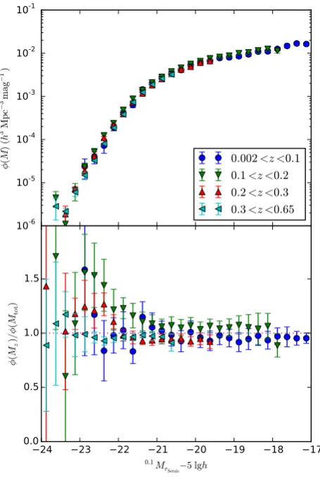
In Fig.9, we investigate how faithfully our simple evolution model, namely one in which log-luminosity and log-density evolve lin-early with redshift, is able to match the GAMA LF measured in redshift slices. The top panel shows Petrosianr-band LFs for the full GAMA-II sample measured in four redshift slices as indicated, calculated using equation (10) with the best-fitting evolution pa-rameters and radial overdensities, and taking into account the ap-propriate redshift limits. If the evolution model accurately reflects true evolution, and if we have successfully corrected for density variations, then these LFs should be consistent where they overlap in luminosity. In the bottom panel, we have divided each LF by the LF determined from the full sample (0.002< z <0.65; top panel of Fig.8) in order to make differences more clearly visible. We see that the lowest redshift LF,z <0.1, is about 10–20 per cent lower than the 0.1< z < 0.2 LF, indicating that the linear

Figure 9. Top panel: Petrosianr-band LFs measured in redshift slices as indicated for the full GAMA sample, applying evolutionary corrections as given in Table3. Bottom panel: the same LFs relative to the overall LF from the top panel of Fig.8.

evolution model is somewhat undercorrecting at the lowest red-shifts. The low-redshift underdensity is particularly severe at the bright end: the most luminous (Mr−5logh−21.5 mag)

galax-ies are underdense by∼50 per cent relative to the higher redshift slices.

Figure 10. As Fig.9but using S´ersic magnitudes.

secondary sources, which introduces a positive flux bias in crowded fields for a small fraction of galaxies, see Section 2.

In conclusion, while the redshift-sliced Petrosian LFs do show some systematic differences, use of GAMA-measured S´ersic mag-nitudes, which capture a larger fraction of total flux for de Vaucouleurs-profile galaxies, and which have an improved back-ground subtraction compared with SDSS DR7, largely mitigates these differences, and suggests that our evolution model is a rea-sonable one.

8 D I S C U S S I O N

8.1 Comparison with previous results

While our evolution-corrected LFs agree well with previous esti-mates, our finding of positive density evolution (in the sense that comoving density was higher in the past) is at odds with most pre-vious work which has tended to find either mildly negative (Cool et al.2012) or insignificant (Blanton et al.2003; Moustakas et al.

2013) density evolution. Faber et al. (2007) find a declining co-moving number density with redshift for their red sample, with no noticeable density evolution for their blue and full samples. Zucca et al. (2009) also find a declining comoving number density with redshift for their reddest sample; for their bluest galaxies, they find increasing number density with redshift.

At least some of the discrepancy between the sign of the density evolution between us and e.g. Cool et al. (2012) might be explained by the way in which the LF and evolution are fitted. Cool et al.

(2012) fit the characteristic magnitudeM∗ to each redshift range using the Sandage et al. (1979) maximum-likelihood method, hold-ing the faint-end slope parameterαfixed at its best-fitting value for the lowest redshift range. They then find the normalizationφ∗ us-ing the Davis & Huchra (1982) minimum-variance estimator. Any overestimate of luminosity evolution would lead to a correspond-ing underestimate in density evolution, due to the assumption of an unchanging faint-end slope with redshift and the strong corre-lation between Schechter parameters. Although any determination of evolution will be affected by degeneracies between luminosity and density evolution, our method makes no assumption about the (unobserved) faint-end slope of the LF at higher redshifts. On the other hand, we do assume a parametric form for evolution.

It is also plausible that the discrepancies between estimated evo-lution parameters are due to the uncertainties in incompleteness correction required when analysing most galaxy surveys. For ex-ample, when we cap our incompleteness-correction weights to 5, we see a reduction in the estimated density evolution parameters. There are likely to be other effects leading to systematic errors in the determination of evolution parameters, which are not reflected in the (statistical) error contours.

A positive density evolution for the All galaxy sample would suggest a reduction in the number of galaxies with cosmic time, either through merging, or due to galaxies dropping out of the sample selection criteria as they passively fade. Neither scenario seems terribly likely; Robotham et al. (2014) see evidence for only a small merger rate in the GAMA sample. Perhaps a more likely explanation is that the apparent density evolution at low redshift is actually caused by a local underdensity, e.g. Keenan, Barger & Cowie (2013) and Whitbourn & Shanks (2014).

8.2 Future work

There are several ways in which the present work can be extended. Having derived density-correctedVmax values for each galaxy,

it is then trivial to determine other distribution functions, such as the stellar mass and size functions, and their evolution. By way of a quick example, in Fig.11we plot the stellar mass function for

low-redshift (z <0.06) GAMA-II galaxies, using the stellar mass estimates of Taylor et al. (2011). In the mass regime where surface-brightness completeness is high, log(M/M)+2 logh8, we find excellent agreement with the earlier estimate from Baldry et al. (2012) using a density-defining population. The upturn seen in the mass function below log (M/M)+2logh≈7 will be sensitive to the incompleteness corrections applied; confirmation of this feature will need to await the availability of deeper VLT Survey Telescope Kilo-degree Survey (VST KiDS) imaging in the GAMA regions. Future work will explore the evolution of the stellar mass function. The density-correctedVmaxvalues will also be used to generate

the radial distributions of random points required to measure the clustering of flux-limited galaxy samples (Farrow et al., in prepara-tion)

We plan to explore the possibility of using the Taylor et al. (2011) stellar population synthesis model fits to GAMA data to derive luminosity evolution parametersQefor individual galaxies. If the

models can predictQewith sufficient reliability, the degeneracy in

fitting for both luminosity and density evolution would be largely eliminated. This would also allow for the fact that galaxies have individual evolutionary histories.

We also plan to incorporate the environmental dependence of the LF into our model. Note that the radial overdensities shown in Fig.6are a poor estimate of the density around each galaxy since they are averages over the entire GAMA-II area within each redshift shell. McNaught-Roberts et al. (2014) present estimates of the LF for galaxies in bins of density within 8h−1_{Mpc spheres.}

We are currently extending density estimation to the full GAMA sample using a variety of density measures (Martindale et al., in preparation).

This main focus of this paper has been to correct the LF and radial density for the effects of evolution, rather than to measure evolution per se. An alternative way of constraining evolution is to measure how the luminosity of galaxies at a fixed space density evolves. Via comparison with a model for the evolution of stellar populations (or luminosity evolution of the Fundamental Plane), one can estimate the rate of mass growth, e.g. Brown et al. (2007).

9 C O N C L U S I O N S

We have described an implementation of the Cole (2011) JSWML method used to infer the evolutionary parameters, the radial density variations and therband LF of galaxies in the GAMA-II survey. For the overall population, we find that galaxies have faded inr-band luminosity by about 0.5 mag, and have decreased in comoving number density by a factor of about 1.6 sincez≈ 0.5, i.e. over the last 5 Gyr or so. When the population is divided into red and blue galaxies, the differences in density evolution parameterPe

are statistically insignificant. Luminosity evolution is significantly stronger for blue galaxies than for red. Evolution in the luminosity density evolution of blue galaxies is higher than that of red at the∼5σlevel. These findings are consistent with those of Loveday et al. (2012) based on GAMA-I and are as expected, since a fraction of galaxies that were blue in the past will have since ceased star formation and become red.

While there still exists some degeneracy between the parameters describing luminosity (Qe) and density (Pe) evolution for GAMA-II

data, see Fig.5, analysis of simulated data and comparison with a local galaxy sample from SDSS (Blanton et al.2005) shows that we are able to recover the evolution-corrected LF to high accuracy. In detail, GAMA LFs are poorly described by Schechter functions,

due to excess number density at both faint and bright luminosities, particularly for the red population.

The density-correctedVmaxvalues will be made available via the

GAMA data base (http://www.gama-survey.org/).

AC K N OW L E D G E M E N T S

JL acknowledges support from the Science and Technology Facil-ities Council (grant number ST/I000976/1) and illuminating dis-cussions with Shaun Cole. PN acknowledges the support of the Royal Society through the award of a University Research Fellow-ship, the European Research Council, through receipt of a Starting Grant (DEGAS-259586) and the Science and Technology Facilities Council (ST/L00075X/1). It is also a pleasure to thank the referee, Thomas Jarrett, for his careful reading of the paper and for his many useful suggestions.

GAMA is a joint European-Australasian project based around a spectroscopic campaign using the Anglo-Australian Telescope. The GAMA input catalogue is based on data taken from the Sloan Digital Sky Survey and the UKIRT Infrared Deep Sky Survey. Com-plementary imaging of the GAMA regions is being obtained by a number of independent survey programmes including GALEX MIS, VST KiDS, VISTA VIKING, WISE, Herschel-ATLAS, GMRT and ASKAP providing UV to radio coverage. GAMA is funded by the STFC (UK), the ARC (Australia), the AAO, and the participating institutions. The GAMA website is:http://www.gama-survey.org/.

R E F E R E N C E S

Abazajian et al., 2009, ApJS, 182, 543

Baldry I. K., Glazebrook K., Brinkmann J., Ivezi´c v., Lupton R. H., Nichol R. C., Szalay A. S., 2004, ApJ, 600, 681

Baldry I. K., Balogh M. L., Bower R. G., Glazebrook K., Nichol R. C., Bamford S. P., Budavari T., 2006, MNRAS, 373, 469

Baldry I. K. et al., 2010, MNRAS, 404, 86 Baldry I. K. et al., 2012, MNRAS, 421, 621 Baldry I. K. et al., 2014, MNRAS, 441, 2440

Bell E. F., McIntosh D. H., Katz N., Weinberg M. D., 2003, ApJS, 149, 289 Benson A., Bower R., Frenk C., Lacey C., Baugh C., Cole S., 2003, ApJ,

599, 38

Bernardi M., Meert A., Sheth R. K., Vikram V., Huertas-Company M., Mei S., Shankar F., 2013, MNRAS, 436, 697

Bertin E., Arnouts S., 1996, A&AS, 117, 393 Blanton M. R., Roweis S., 2007, AJ, 133, 734 Blanton M. R. et al., 2001, AJ, 121, 2358 Blanton M. R. et al., 2003, AJ, 125, 2348

Blanton M. R., Lupton R. H., Schlegel D. J., Strauss M. A., Brinkmann J., Fukugita M., Loveday J., 2005, ApJ, 631, 208

Blanton M. R., Kazin E., Muna D., Weaver B. A., Price-Whelan A., 2011, AJ, 142, 31

Brown M. J. I., Dey A., Jannuzi B. T., Brand K., Benson A. J., Brodwin M., Croton D. J., Eisenhardt P. R., 2007, ApJ, 654, 858

Cole S., 2011, MNRAS, 416, 739 Cool R. J. et al., 2012, ApJ, 748, 10 Davis M., Huchra J., 1982, ApJ, 254, 437 Driver S. P. et al., 2011, MNRAS, 413, 971 Driver S. P. et al., 2013, MNRAS, 427, 3244

Efstathiou G., Ellis R. S., Peterson B. A., 1988, MNRAS, 232, 431 Ellis S. C., Bland-Hawthorn J., 2007, MNRAS, 377, 815 Faber S. M. et al., 2007, ApJ, 665, 265

Hill D. T. et al., 2011, MNRAS, 412, 765

Keenan R. C., Barger A. J., Cowie L. L., 2013, ApJ, 775, 62 Kelvin L. S. et al., 2012, MNRAS, 421, 1007

Lin H., Yee H. K. C., Carlberg R. G., Morris S. L., Sawicki M., Patton D. R., Wirth G., Shepherd C. W., 1999, ApJ, 518, 533

Loveday J., Peterson B. A., Efstathiou G., Maddox S. J., 1992, ApJ, 390, 338

Loveday J. et al., 2012, MNRAS, 420, 1239

McNaught-Roberts T. et al., 2014, MNRAS, 445, 2125 Montero-Dorta A. D., Prada F., 2009, MNRAS, 399, 1106 Moustakas J. et al., 2013, ApJ, 767, 50

Norberg P. et al., 2002, MNRAS, 336, 907

Peebles P. J. E., 1980, The large-scale Structure of the Universe. Princeton Univ. Press, Prineton, NJ

Peng Y.-j. et al., 2010, ApJ, 721, 193 Petrosian V., 1976, ApJ, 209, L1

Robotham A. S. G. et al., 2014, MNRAS, 444, 3986 Sandage A., Tammann G. A., Yahil A., 1979, ApJ, 232, 352

Saunders W., Rowan-Robinson M., Lawrence A., Efstathiou G., Kaiser N., Ellis R. S., Frenk C. S., 1990, MNRAS, 242, 318

Schechter P., 1976, ApJ, 203, 297

Schlegel D. J., Finkbeiner D. P., Davis M., 1998, ApJ, 500, 525 Schmidt M., 1968, ApJ, 151, 393

S´ersic J. L., 1963, Bol. la Asoc. Argentina Astron. La Plata Argentina, 6, 41 Stoughton C. et al., 2002, AJ, 123, 485

Taylor E. N. et al., 2011, MNRAS, 418, 1587 Taylor E. N. et al., 2015, MNRAS, 446, 2144

Tonry J. L., Blakeslee J. P., Ajhar E. A., Dressler A., 2000, ApJ, 530, 625 Whitbourn J. R., Shanks T., 2014, MNRAS, 437, 2146

Zucca E. et al., 2009, A&A, 508, 1217