University of Warwick institutional repository: http://go.warwick.ac.uk/wrap
A Thesis Submitted for the Degree of PhD at the University of Warwick
http://go.warwick.ac.uk/wrap/3788
This thesis is made available online and is protected by original copyright.
Please scroll down to view the document itself.
Robust Surface Modelling of
Visual Hull from Multiple
Silhouettes
by
Dongjoe Shin,
BSc
,
MSc
A thesis submitted in partial fulfillment of
the requirements for the degree of
Doctor of Philosophy
Contents
1 Introduction 1
1.1 Introduction . . . 1
1.2 Vision-based 3D reconstruction . . . 2
1.2.1 Stereo reconstruction . . . 2
1.2.2 Active vision . . . 3
1.2.3 Shape from silhouettes . . . 4
1.3 Major contributions . . . 5
1.4 Thesis organisation . . . 5
2 Shape from Silhouettes 8 2.1 Introduction . . . 8
2.2 Geometric entities in SfS . . . 9
2.3 Visual hull representation . . . 12
2.3.1 Octree representation . . . 12
2.3.2 Silhouette detection . . . 14
2.3.3 Octree construction . . . 19
2.3.4 Status decision in 3D space . . . 25
2.3.5 Experimental results . . . 25
2.4 SfS without an octree . . . 33
2.4.1 Parallelogram and pillar representation . . . 33
2.4.2 3D line segment representation . . . 34
2.5 Visual hull from colour information . . . 34
2.5.2 Voxel colouring . . . 36
2.5.3 Space carving . . . 37
2.5.4 Pros and cons . . . 37
2.6 Conclusions . . . 38
3 Projection transform estimation from circular motion 39 3.1 Introduction . . . 39
3.2 Camera calibration . . . 41
3.2.1 Projection models . . . 41
3.2.2 Camera calibration . . . 43
3.3 Circular Motion . . . 48
3.3.1 Projection matrix and cost function of SfS . . . 48
3.3.2 Fixed entities in a circular motion . . . 50
3.4 Modified projection matrix for an approximate circular motion . . . 53
3.5 Experimental results . . . 55
3.6 Conclusions . . . 59
4 Feature correspondences from wide baseline views 62 4.1 Introduction . . . 62
4.2 Delaunay graph . . . 63
4.3 Similarity invariant graph matching . . . 67
4.3.1 Point pattern matching . . . 67
4.3.2 Clique distance . . . 69
4.3.3 Guided matching . . . 72
4.4 Clique descriptor matching . . . 74
4.4.1 Feature descriptor matching . . . 74
4.4.2 MSER detector . . . 75
4.4.3 IR descriptor . . . 77
4.4.4 Clique descriptor . . . 77
4.4.5 Clique descriptor distance . . . 80
4.5 Experimental results . . . 82
4.5.2 Clique descriptor matching . . . 86
4.6 Conclusions . . . 90
5 Visual hull refinement 94 5.1 Introduction . . . 94
5.2 Epipolar transfer . . . 96
5.3 Image calibration algorithm . . . 99
5.4 Experimental results . . . 100
5.5 Conclusions . . . 106
6 Robust surface modelling 108 6.1 Introduction . . . 108
6.2 Surface from silhouettes . . . 110
6.2.1 Marching cubes and its variants . . . 110
6.2.2 Delaunay triangulation and convex hull . . . 113
6.3 Overview of the proposed method . . . 115
6.4 Local hull-based surface construction . . . 118
6.4.1 Volumetric data slicing . . . 118
6.4.2 Identifying a local convexity . . . 121
6.4.3 Local surface construction . . . 125
6.4.4 Implementation . . . 130
6.5 Experimental results . . . 130
6.6 Conclusion . . . 138
7 Conclusion and future work 141 7.1 Conclusions . . . 141
7.2 Future work . . . 144
A List of publications 146 B Preliminary projective geometry 147 B.0.1 Geometric primitives in 2D projective space . . . 147
B.0.3 Two-view geometry . . . 152
C Singular value decomposition 154
D Hausdorff distance and its variants 156
D.1 Traditional HD . . . 156
D.2 Useful variations of HD . . . 157
E Robust regression 158
F Programming naming conventions 160
F.1 C++ and C . . . 160
List of Figures
2.1 Shape from Silhouette approach: Three views with camera centre!cw i ,!cw(i−1)
and!cw
(i+1)produce silhouette cones and intersections (e.g.,!pw1,!p2w,!pw3,!pw4,
and !pw
5) approximate the volume of an object. Dotted lines on the object
denote each contour generator and frontier points are marked as triangle,
circle and square. . . 10
2.2 Example of an octree: (a) Grey voxels indicates the actual shape of an object, whilst dotted cubes represent the shape of octants. The indices correspond to the node indices in the second level of octree in (b); (b) A three-level of an octree of the object shown in (a), where black, white and grey node represent inside, background and intersection octant, respectively. 13 2.3 Size filtering code snippet 1. . . 16
2.4 Size filtering code snippet 2. . . 17
2.5 Example of silhouette detection: (a) objects with non-homogeneous tex-ture; (b) thresholding result of (a); (c) a silhouette is estimated by applying the flood-seeding algorithm to the largest occluding contour; (d) an object with homogeneous texture but two internal cavities; (e) two inside holes cannot be distinguishable after the food-seeding algorithm; (f) two internal segments complete the silhouette detection. . . 18
2.6 COctant declaration snippet 3 . . . 20
2.7 Octree construction method I snippet 4. . . 21
2.8 Octree construction method II snippet 5. . . 22
2.9 Intersection test snippet 6. . . 24
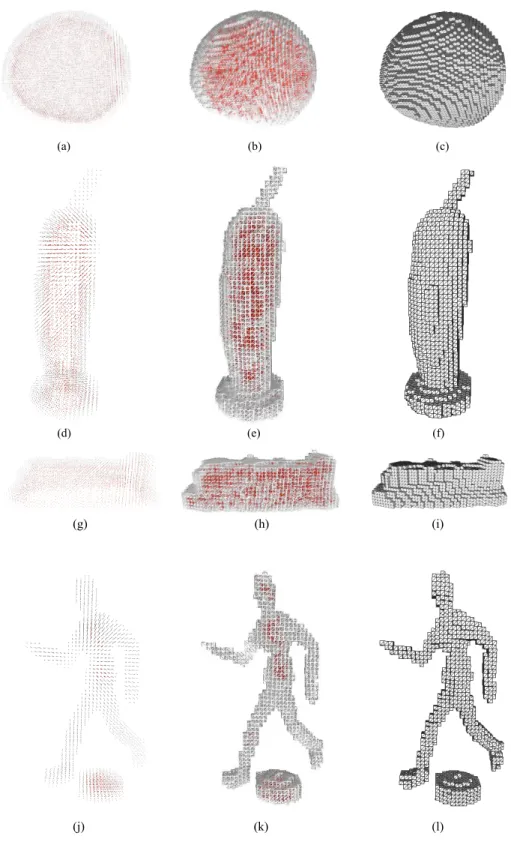
2.11 Reconstruction results: (a)-(c) reconstruction results of the object shown
in Figure 2.10(a); (d)-(f) reconstruction results of the object in Figure
2.10(b); (g)-(i) reconstruction results of the object in Figure 2.10(c); (j)-(l)
reconstruction results of the object in Figure 2.10(d); Each reconstruction
is presented as point view, wireframe view and face view in three columns,
and internal octants are highlighted in red. . . 27
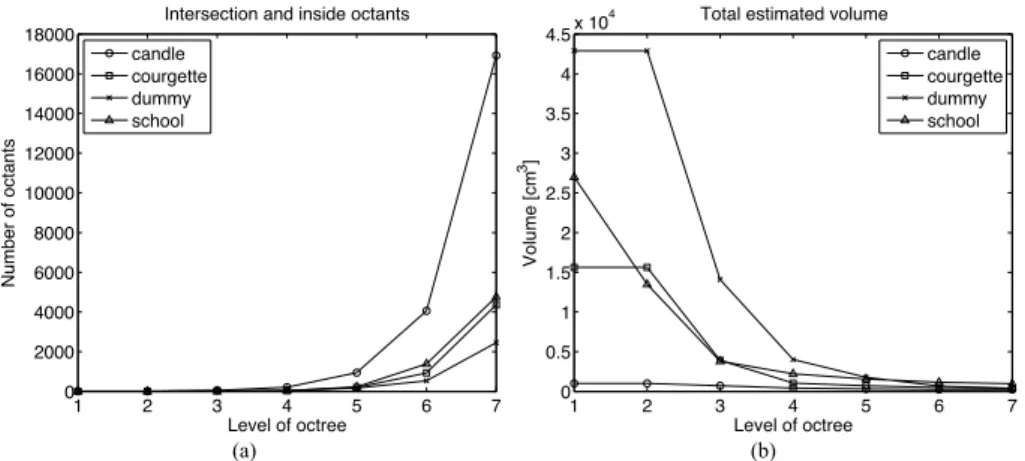
2.12 Total octants and volume of four objects: (a) total number of octant; (b)
its volume relative to the level of an octree. . . 28
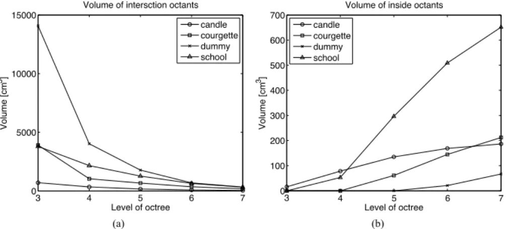
2.13 Inside and intersection volume: (a) intersection volume and (b) inside
vol-ume relative to the level of an octree. . . 29
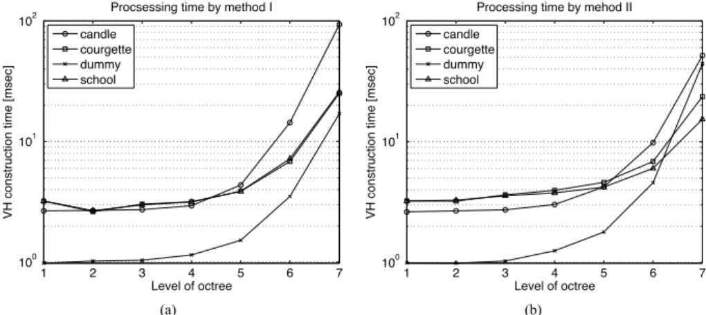
2.14 Processing time of two methods: (a) result of method I and (b) method II.
The vertical axes of both graphs are log scaled. . . 30
2.15 Intermediate results of the progressive reconstruction of the dummy shown
in Figure 2.10(d): Each image from (a) to (g) corresponds to the 1 to
7-level of octree construction. . . 31
2.16 VH results relative to viewing directions: (a) result using 15 images equally
spaced at a quarter of a rotation; (b) result using four images from the main
diagonal directions in the xy plane of a world frame; (c) result using 60
images of the rotated object. . . 32
3.1 Calibration performance: (a)-(c) three test images of a calibration
pat-tern, where + denotes a 2D point used for the calibration; (d) average
re-projection errors of DLT solutions obtained from (a), (b) and (c). . . . 47
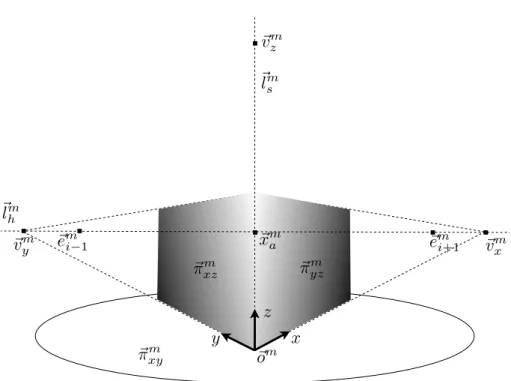
3.2 Example of fixed entities of a circular motion: a vanishing line of axyplane
(!lm
h) and an image of a screw axis (!lms ) are unchanged over all images in
a circular motion. Additionally, three points on a rotation axis are also
invariant, e.g.,!vm
3.3 Example of estimation error of a circular motion: (a) average re-projection
error of projection matrices estimated from a pure circular motion with
respect to rotation angle; (b) true * and estimated camera centres!in a
world frame, where the reference camera position is connected to the origin
of world frame ◦. . . 52
3.4 Geometrical illustration of a circular motion. . . 54
3.5 Average projection error before and after the projection modification. . . 56
3.6 Example of two fixed lines in a pure circular motion: (a) the difference of
true and approximated fixed line entities are noticeable due to additional
3D translation; (c) although two fixed lines entities are almost identical,
the projection error is high for points further away from the rotation axis,
i.e., additional rotation is involved in thez axis; (b) and (d) the modified
image planes are denoted by white boundary. . . 58
3.7 Example of modified images for the volumetric reconstruction by a SfS
technique. White boundary in each image illustrates an image of a true
image plane in an estimated view. . . 60
4.1 (a) A Voronoi diagram of 20 feature points (denoted by *) that are
ran-domly generated and ranged [0 1]. (b) A Delaunay graph, the dual of the
Voronoi diagram in (a). (c) The general shape of Delaunay graph in (b) is
not changed by the addition of a noise point o. (d) A randomly selected
small portion of features does not change the local graph significantly. . . 65
4.2 Example of a clique: (a) a model cliqueCim; (b) a test cliqueCjt, where!vi
and!vj are the seeds of the cliques. . . 66
4.3 Pseudo code for a 2D Delaunay graph construction. . . 66
4.4 Illustration of a geometrical distance: (a) a triangle defined by (!v7, !vn7,2, !vn7,3)
is a face ofC7 and its cross ratio isfcr(!vn7,2, !µ
1! 7,2, !µ2
!
7,2, !vn7,3); (b) for a face
(!v9, !vn9,2, !vn9,3) with an obtuse angle, the projection of a midpoint is
4.5 (a) Noise points (denoted by o) and signal points (denoted by *). (b)
Solid line represents the Delaunay graph of the signal points only; dashed
graph represents the Delaunay graph due to the noise points; and strong
correspondences are denoted by *. . . 73
4.6 Example of MSER detection: (a) A detected MSER is illustrated as an
ellipse and a cross represents the centre of the ellipse; (b) Textured MSER
of (a); (c) MSER of (a); (b) and (c) are represented in a normalised patch of
whichNp= 41; (d) The SIFT description of (b) and (c) are represented by
a dashed line with a square mark and a solid line with a cross, respectively. 78
4.7 A clique descriptor: (a) a Delaunay graph determined by local reference
frame of the 254-th MSER; (b) 7 neighbours of seed 254 in a clique,
where T.M. represents a textured MSER; (c) and (d) show angle values
in A254(254) and size valuesZ254(254) . . . 81
4.8 (a) The 251 model points extracted from the 348×360 image for partial
matching are denoted by +, with their Delaunay graph overlaid. (b) The
selected data is bounded by the solid reference line and the dashed sweeping
line with θs= 60◦. (c) Normalised matching distances of HD, MHD, 30%
RHD, 50% RHD, 70% RHD and clique HD, are respectively denoted by
!,◦, x, +,•and *. . . . 84
4.9 Test images for evaluating the identification capability: (a) china 1; (b)
china 2; (c) remote controller; and (d) a graph generated by rotating (a)
by 45◦ and random translation. . . . 85
4.10 Matching images from different views: (a) Result of equally weighted clique
descriptor matching using textured MSER’s; (b) Inliers from matching
using: EWC descriptor (!), AWC descriptor (∆), a pair descriptor (◦),
SIFT (x) and correlation (*). A solid and dashed lines denote matching
result of textured MSER’s and MSER’s, respectively. . . 87
4.11 Matching images with homogeneous texture from different views: (a)
Re-sult of equally weighted clique descriptor matching using textured MSER’s;
(b) Inliers from matching using 3 group descriptors, SIFT and correlation
4.12 Matching two images one of which with zoom and rotation: (a) Result of
the equally weighted clique descriptor matching using textured MSER’s;
(b) Inliers from matching using 3 group descriptors, SIFT and correlation
denoted using the same symbols in Figure 4.10(b). . . 91
4.13 Examples of matching images generated from a circular motion: (a) images
at 0◦to 40◦; (b) textured MSER based matching results using correlation,
SIFT, Pair, AWC and EWC. . . 92
5.1 Geometry of an image triplet: given a point correspondence !x(i−1) ↔
!x(i+1), the linear triangulation can infer its 3D position!xw by intersecting
two rays back-projected from the corresponding points (see dotted arrow
on an epipolar plane!πw
e). Furthermore, when two fundamental matrices
F12 and F32 are known, an image of!xw in an additional imageIi can be
determined without a projection matrix by the intersection of two epipolar
lines. . . 97
5.2 Example of a degenerate epipolar transfer: three images (a), (b), and (d)
are captured in a circular motion, and (a) and (c) are images captured
at the same rotational angle. Two epipolar lines associated with a point
marked as ‘+’ in (b) and (d) are represented as a white line in (a) and (c).
Those two lines are parallel, so that an intersection of two epipolar lines
cannot locate a matching point. . . 98
5.3 An algorithm for the image calibration from an image triplet. . . 99
5.4 (a) Images added to VH construction across time t(n), where n= 1,2,3;
(b) VH’s (the first row) and their surface mesh (the second row) generated
using 3 views and with added images. The reference VH and surface meshes
5.5 (a) and (c): Two initial images taken from a circular motion with +
de-noting matched MSER centres; (b) An additional image with the
corre-sponding points in the initial images; (d) and (e) are point matching result
for estimating two fundamental matrices; (f) 3D positions of corresponding
points, and camera positions for images in (a), (b) and (c) are respectively
marked as !, ◦ and *; (g) Projection of the initial VH of a spray onto
the new image, where dots represents voxel corners and lines visualise a
convex hull defined from dots; (h) Initial VH constructed from four images
including the initial images; (i) Improved VH by adding the new image. . 104
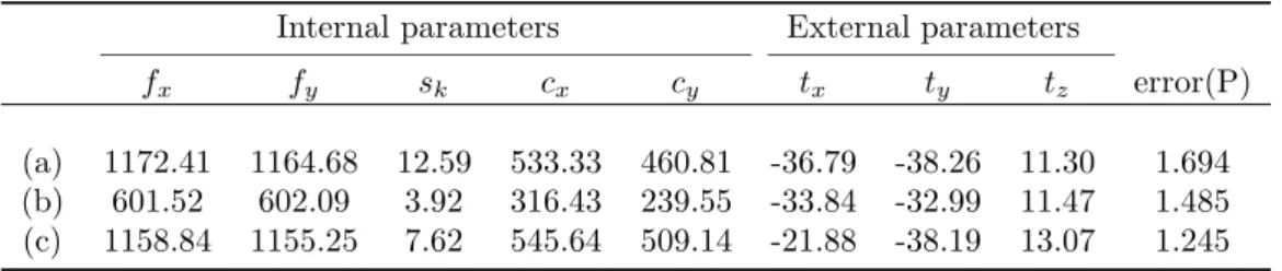
5.6 Calibration test: (a) and (b) initial images with known projection
matri-ces; (c)-(f): images with unknown projection matrices. The intrinsic and
extrinsic parameters of the camera for the images (c)-(f) are listed in Table
5.2 . . . 105
6.1 Example of three intersection cases : (a) case a; (b) case b; (c) case c. A
polygon with grey shade represents a silhouette and a cube is formed from
eight projection points. . . 112
6.2 Voting estimation. . . 113
6.3 Example of VMC results relative toτv: (a) voting threshold is set toτv =
m, which is equivalent to mc result; (b)τv = 0.9m; (c)τv = 0.8m; (d)τv =
0.7m. Three axes represents three bases of world fame and the unit is [cm]. 114
6.4 Convex hull Vs 3D Delaunay from randomly generated 100 3D points: (a)
convex hull does not use all points to construct triangle patches but the
result is always convex; (b) all points are connected by triangle edges and
result also forms a convex. . . 116
6.5 The overall surface construction process. . . 117
6.6 (a)Ioc
i where ‘×’ and ‘◦’ respectively represent a vertex of an intersection
octant and internal octant ini-th octree slice. (b)Ioc
i where total number
6.7 (a) Examples of silhouettes obtained using simple thresholding, which
pro-duces imperfect occluding contours. (b) A seven-level of octree from sixty
silhouette images. (c) The best surface result from VMC with 85% voting
threshold. The unit of three axes in (b) and (c) is [cm]. . . 122
6.8 Examples of slicesIiocq where each slice is quantised as 28×28 grid, where a nonzero value on a slice represents an octant. . . 123
6.9 Examples of pdf cubes: a 3D pdf cube contains every cluster conditional
pdf found in a quantised octree slice. A cluster conditional pdf interpolates
110x110 pixels and the size of the Gaussian window is 3. . . 126
6.10 1:nbranching case. If the 3D hull algorithm is simply applied to multiple
connections, some object details will be smoothed. To avoid the smoothing,
the clusterc1is divided into 3 subregions,R2,R3andR4on the projection
of the eigen vectorV# and n1:1 connections are made. . . 128
6.11 Surface generation. . . 130
6.12 Eight-level octrees and MC surfaces of four test objects: (a)-(d) Images of
objects at the reference position; (e)-(h) The corresponding octrees
respec-tively with 362320, 75504, 267072 and 378448 octants; (i)-(l) MC surfaces
from (e)-(h). . . 132
6.13 (a)-(d) Silhouette images with 10% noise added; (e)-(f) MC surfaces
esti-mated from silhouette images with 5% noise added; (i)-(l) the best VMC
results from silhouette images with 10% noise added. . . 134
6.14 (a) Lost octants ratios using MC for varying noise ratios. (b) Lost octants
ratios using VMC for varying voting thresholds. . . 135
6.15 Surface reconstruction from the best VMC result: (a)-(d) using the convex
hull algorithm; (e)-(h): using the proposed method. . . 136
6.16 (a) CPU time and (b) peak memory usage required by 6 algorithms to
construct 4 objects. . . 137
6.17 (a)-(c) A dummy with different poses. (d)-(f) The corresponding silhouette
images using simple thresholding. (g) seven-level octree. (h) MC surface.
6.18 Octree, MC, VMC, and LCH results of (a) the dummy; (b) a school model
List of Tables
2.1 Octree updating rule. . . 14
2.2 VH relative to viewing directions. . . 33
3.1 Camera parameters from DLT solution. . . 48
3.2 Camera parameters from LM solution. . . 48
3.3 Seven-level volume reconstruction result before and after modification of projection matrices. . . 57
3.4 Eight-level volume reconstruction result before and after modification of projection matrices. . . 59
4.1 Identification test results. . . 86
5.1 VH’s created using different number of additional images. . . 102
5.2 Estimated camera parameters from DLT Vs. the proposed method . . . . 106
6.1 VMC surface construction result . . . 113
6.2 Connection tree. . . 127
Acknowledgements
I would like to take this opportunity to thank my research supervisor Dr. T. Tjahjadi for
his academic and financial support towards this research. I would also like to express my
gratitude to the annual progress panels in the School of Engineering: Dr. R. Staunton,
Dr. N. Stocks, and Prof. J. Gardner. Their kind advice about the research was a constant
help. Finally, I would like to thank my fellow students (and now Drs) for their support,
Declaration
This thesis is submitted in partial fulfilment for the degree of Doctor of Philosophy under
the regulations set out by the Graduate School at the University of Warwick. This thesis
is solely composed of research undertaken by Dongjoe Shin under the supervision of
Dr. Tardi Tjahjadi. The research materials have not been submitted in any previous
application for a higher degree. All sources of information are specifically acknowledged
Abstract
Reconstructing depth information from images is one of the actively researched themes
in computer vision and its application involves most vision research areas from object
recognition to realistic visualisation. Amongst other useful vision-based reconstruction
techniques, this thesis extensively investigates the visual hull (VH) concept for volume
approximation and its robust surface modelling when various views of an object are
available. Assuming that multiple images are captured from a circular motion, projection
matrices are generally parameterised in terms of a rotation angle from a reference position
in order to facilitate the multi-camera calibration. However, this assumption is often
violated in practice, i.e., a pure rotation in a planar motion with accurate rotation angle
is hardly realisable. To address this problem, at first, this thesis proposes a calibration
method associated with the approximate circular motion.
With these modified projection matrices, a resulting VH is represented by a
hi-erarchical tree structure of voxels from which surfaces are extracted by the Marching
cubes (MC) algorithm. However, the surfaces may have unexpected artefacts caused by
a coarser volume reconstruction, the topological ambiguity of the MC algorithm, and
imperfect image processing or calibration result. To avoid this sensitivity, this thesis
proposes a robust surface construction algorithm which initially classifies local convex
regions from imperfect MC vertices and then aggregates local surfaces constructed by the
3D convex hull algorithm. Furthermore, this thesis also explores the use of wide baseline
images to refine a coarse VH using an affine invariant region descriptor. This improves
the quality of VH when a small number of initial views is given.
In conclusion, the proposed methods achieve a 3D model with enhanced
accu-racy. Also, robust surface modelling is retained when silhouette images are degraded by
Abbreviations
2D Two Dimensional
3D Three Dimensional
AI Artificial Intelligence
B-Rep Boundary Representation
CAD Computer Aided Design
CCD Charge-Coupled Device
CDT Constrained Delaunay Triangulation
CSG Constructive Solid Geometry
DLT Direct Linear Transformation
DoF Degree of Freedom
DT Delaunay Triangulation
HD Hausdorff Distance
IR Invariant Region
LM Levenberg-Marquardt
LMS Least Mean Square
LMedS Least Median Square
MHD Modified Hausdorff Distance
MSER Maximum Stable Extremal Region
NN Neural Networks
pdf probability density function
PH Photo Hull
PPM Point Pattern Matching
RANSAC RANdom SAmple Consensus
SC Space Carving
SfS Shape from Silhouette
SIFT Scale Invariant Feature Transform
STL Standard Template Library
SVD Singular Value Decomposition
VC Voxel Colouring
Chapter 1
Introduction
1.1
Introduction
Computer vision is an inter-disciplinary subject that investigates a decision-making
al-gorithm based on the analysis of digitised images. Thus, it is highly related to image
processing, pattern recognition and photogrammetry which are concerned with obtaining
reliable and accurate measurements from non-contact imaging [1], and are often
moti-vated by biological vision and psychophysics [2]. An image is a vital source of significant
visual information for recognition (e.g., the colour and shape of an object), on which
re-cent vision systems heavily rely. More specifically, these systems exploit distinctive image
features, which are extracted from the visual clues and incorporated in a sophisticated
decision making scenario generally devised from Artificial Intelligence (AI), Neural
Net-work (NN) theory, and statistical analysis. Indeed, this approach retains a certain level
of recognition performance.
However, it is inevitable that a feature defined on the projection of a 3D object is
deprived of the information from the higher dimension, so that these clues can be sensitive
to viewing conditions. For example, the shape can be distorted by viewing directions,
and colour can change according to the material of an object, lighting condition and the
sensor characteristic. Consequently, there are some limits to understand 3D scene solely
based on 2D image features. To address this limited capability of traditional 2D features,
features, and this thesis is also inspired by the concern regarding how to obtain accurate
shape information from multiple images in a robust way.
This introduction chapter is organised as follows. Section 1.2 briefly reviews
fundamental ideas of conventional vision-based 3D reconstructions, such as stereo camera,
shape from silhouettes and active vision techniques. Section 1.3 shows a list of major
contribution. The last section presents the outline of the thesis.
1.2
Vision-based 3D reconstruction
There are various approaches to reconstructing a 3D object or scene from images. This
section briefly explains three major methods (e.g., stereo reconstruction, active vision,
and shape from silhouettes) and identifies pros and cons of each approach.
1.2.1
Stereo reconstruction
Stereo reconstruction is inspired by human stereopsis, i.e., perceiving depth from
binocu-lar disparity. The realisation of this mechanism requires two cameras and the
reconstruc-tion performance is superior to that from monocular visual clues, such as texture and
shading1. Given a pair of 2D corresponding points associated with two projection
ma-trices, a stereo reconstruction computes a depth of the 2D point from a triangle, formed
by a camera baseline and an intersection point of two back-projection rays from the pair
of corresponding points. Therefore, the primary concerns in early stereo reconstruction
research are: how to estimate point correspondences accurately and efficiently in
prac-tical situations, where a matching point often disappears by occlusion in another view
[8, 6]; and how to minimise the triangulation error when physical lens characteristics do
not comply with a linear calibration result [1, 9]. Therefore, most of early researches try
to achieve robust image matching and to search for an appropriate non-linear projection
model compensating a linear estimation of a projection matrix. Recently research effort
has moved to self-calibration techniques which determines projection matrix only from
1
image correspondences so that the reconstruction is realised without an offline camera
calibration.
The shape from stereo method produces a reliable depth result. However, the
result is generally given as a form of unorganised point cloud, which further requires
a surface generation algorithm for realistic visualisation. The density of reconstructed
points is not consistence, e.g., objects with homogeneous texture suffer lack of feature
points. Furthermore, the volume of an object cannot be determined from only two views
placed in front of the object. Therefore, it is unable to extract significant 3D information,
such as surface curvature, surface normal vectors, and the volume of a certain region.
1.2.2
Active vision
Active vision includes all shape reconstruction methods that exploit an image of an object,
on which an external energy (e.g., a laser or a light projector) is intentionally projected
to alleviate the problems occurring in traditional stereo techniques. Fundamentally, it is
a case that the second camera is replaced with a laser projector, so that the
reconstruc-tion is more actively achieved by means of more than visual informareconstruc-tion. As an accurate
energy source, the early active vision mostly utilises a laser, though it has been replaced
with a practical light projector later. For example, a line generated from a laser scans
an object and images captured during scanning produce 3D information after an active
triangulation, which is a modification of the traditional triangulation to exploit the scene
geometry established from a projector and a camera [2]. Consequently, this line-sweeping
produces sufficient number of feature points even in a textureless object and establishing
point correspondences is no longer required in the reconstruction process. Furthermore,
surfaces of the reconstructed points are straightforwardly constructed from the skinning
algorithm [10]. To reduce the scanning time, multiple lines are often projected
simul-taneously in a binary coded pattern [2]. However, this approach requires to analyse a
sequence of scanned images spatio-temporally, e.g., each image is processed to extract
distorted line segments (an image of projected lasers) and they are classified by images
captured at other time instances. As an alternative of a rapid reconstruction, all sweeping
lines are encoded into a special pattern called a coded light pattern to realise the one-shot
A major disadvantage of an active system is that it needs to be equipped with
a precise light projecting source, which is not cost efficient, and the object has to stay
still when a line sweeps. Although a specially coded pattern can ease some constraints,
it involves a pattern decoding process which is similarly complex as the correspondence
problem in a stereo reconstruction. However, because of the high accuracy, it is mostly
adopted in industrial applications.
1.2.3
Shape from silhouettes
Shape from Silhouette (SfS) retrieves volume information from multiple images, where
the images do not need to be correlated with each other by an underlying motion, such
as a sequence used in the structure from motion technique. Instead of the triangulation,
the volume of an object is approximated by the intersections of cones, defined by a set
of back-projection rays on an object boundary. Therefore, complicated point detection
and matching processes are reduced to a silhouette image detection, i.e., it only utilises
the information on whether a 2D image location is occupied by an object. The quality
of the reconstructed volume relies on the viewing directions as well as the number of
image used, so that it is better for multiple images to surround an object, although a
rough approximation of the volume is still possible from a few shots at widely separated
positions. Once the volume data is approximated, the construction of the object surface
is much easier, e.g., using the marching cubes algorithm [12] to extract triangular meshes
from cubic volume elements. The quality of surface meshes is adaptively controlled in
recent variants of marching cubes [13].
A silhouette presents an object as binary values in an image plane, i.e., white
rep-resents a pixel occupied by an object and black is not occupied. Therefore, SfS techniques
search for voxels (i.e., volume elements) not belonging to the silhouette and discard them
to confine the object volume. Later developments of SfS technique exploit the colour
consistency of a scene in a carving procedure. Thus, such an approach does not requires
image segmentation for silhouette detection (which is not reliable in a cluttered scene),
and the texture of object surface is simultaneously determined during the volume
recon-struction. However, the colour consistency is only acceptable when a large number of
the number is increased.
Each of three major vision-based reconstruction techniques has its own advantages
and disadvantages so that the reconstruction is appropriately chosen according to its
application area. Since this thesis explores a shape reconstruction as a potential 3D
source of an object recognition system, a SfS method, which is solely based on images but
constructs volume information without the complex matching process, is mainly explored.
1.3
Major contributions
The main contribution of this thesis is delivering a robust 3D modelling algorithm which
exploits volume information obtained from multiple images of an object. To realise this
goal, this thesis also investigates the following sub-research topics:
• multiple camera calibration from approximated circular motion;
• VH improvement from additional uncalibrated images;
• robust surface modelling from a volume data.
In particular, state-of-the-art image matching algorithms including image region
descrip-tor are thoroughly explored to achieve the wide-baseline image matching, which plays a
key role when tackling problems of the above topics. However, the proposed method is
currently limited to static scene application with a controlled background.
1.4
Thesis organisation
This thesis contributes to the accurate 3D volume recovery from multiple views and its
visualisation. To achieve this, the thesis explores five different research topics: volume
reconstruction, projection matrix modelling, robust image matching, visual hull
improve-ment and surface construction from volume data. Consequently, each chapter from
Chap-ter 2 to ChapChap-ter 6 has been written as an independent work, which aims to the same
goal. Brief explanation of each chapter are as follows.
Chapter 2 presents a detailed explanation of the volume reconstruction technique,
silhouette cone and frontier point), and octree representation of a volumetric data. Some
pseudo codes and code snippets are presented to illustrate the silhouette detection and
octree construction. In addition, this chapter analyses reconstruction results of objects
with different shape complexity. Also, the latest approaches in SfS, the voxel colouring
and space carving algorithms, are reviewed and compared to a traditional SfS.
Chapter 3 presents a 3D object reconstruction system which uses multiple images
taken with a fixed camera of an object moving in an approximate circular motion. The
circular motion is generally defined to be a pure rotation case of planar motion when
modelling a turntable image sequence or equivalently an image sequence of a fixed object
generated with a rotating camera. However, in practical situations the assumption of pure
rotation is often violated as the rotation axis is not fixed during the rotation of a turntable.
To address this problem, this chapter proposes a modified method for estimating the
projection matrix associated with circular motion and an object reconstruction method
based on the octree algorithm. Experimental results on several real turntable image
sequences demonstrate good object reconstructions.
Chapter 4 proposes a robust image matching method. Establishing point
corre-spondences between images is a fundamental process in many computer vision
applica-tions, e.g., motion tracking, auto calibration and object recognition. In particular, this
thesis exploits it for the visual hull refinement. Before introducing the refinement
algo-rithm, this chapter proposes two matching methods associated with Delaunay tessellation
and Hausdorff distance. Delaunay tessellation describes a set of arbitrarily distributed
points as unique triangular graphs which preserves most local point configuration called
a clique regardless of noise addition and partial occlusion. In this chapter, this structure
is utilised in a matching method and a clique-based Hausdorff Distance (HD) to address
point pattern matching problems is proposed. Moreover, to enhance matching
perfor-mance under affine transform, a feature descriptor, a distinctive and compact form of
local information near to a feature point, is incorporated in the point pattern matching
and a clique descriptor is introduced as a result.
Chapter 5 explains an algorithm that enhances the volume reconstruction from
additional images. The quality of a Visual Hull (VH) depends on the number of silhouette
which improves an initial coarse VH by using additional images captured at arbitrary
positions with unknown camera parameters. The method calibrates a new image from
3D-to-2D point pairs which are obtained by epipolar transfer of two initial images and a
new image, and stereo based point reconstruction.
Chapter 6 is about a robust surface construction method using volume data. The
Marching Cube (MC) is a general method which can construct a surface of an object
from its volumetric data generated using a shape from silhouette method. Although MC
is efficient and straightforward to implement, a MC surface may have a discontinuity
even though the volumetric data is continuous. This is because surface construction is
more sensitive to image noise than the construction of volumetric data. To address this
problem, this chapter proposes a surface construction algorithm which aggregates local
surfaces constructed by the 3D convex hull algorithm. Thus, the proposed method initially
classifies local convex regions from imperfect MC vertices based on sliced volumetric data.
Experimental results show that continuous surfaces are obtained from imperfect silhouette
images of both convex and non-convex objects. Finally, Chapter 7 summarises the thesis
Chapter 2
Shape from Silhouettes
2.1
Introduction
Traditional scene reconstruction from stereoscopic images requires a robust feature
match-ing process and restricts the length of a baseline of the two views (e.g., too narrow baseline
degrades the accuracy of triangulation), in order to obtain an appropriate number of 3D
points with good accuracy. Furthermore, in case where there are only sparse features
due to the homogeneous texture of the object, it is necessary to perform parameterised
surface modelling to interpolate surfaces in order to increase the density of reconstructed
points. After all, the most challenging task in stereo reconstruction is to solve the feature
matching problem explicitly in an occluded view, even though many algorithms have been
introduced to address this issue.
However, when the surrounding views of an object and projection transforms are
available, the volume of an object can be confined by the intersections of silhouette cones
without point correspondences, resulting in a 3D convex hull called a Visual Hull (VH)
[14]. This approach is sometimes called the volume intersection technique, but
recon-struction methods involving projection (or back-projection) of multiple silhouettes are
collectively referred to as the Shape from Silhouette (SfS) technique. Therefore, SfS is
more robust than stereoscopic reconstructions and it can control the density of surface
meshes as they depend on the predefined voxel resolutions. This chapter explains the
cone, followed by the introduction of two useful VH construction schemes. It also
anal-yses the reconstruction performance of four objects with different shape complexity and
discusses some implementing issues. Therefore, this chapter mainly explores the following
topics:
• the geometric aspect of of Shape from Silhouette technique;
• two straightforward silhouette detection algorithms;
• a general implementation of octree reconstruction in addition to two bespoke
algo-rithms developed for the thesis experiments;
• brief review of relevant researches (i.e., various volume representations) and recent
variations of SfS such as voxel colouring and space carving.
2.2
Geometric entities in SfS
The basic approach of reconstruction by volume intersection is dated back to Baumgart’s
1974 PhD thesis, where a polyhedral visual hull is constructed by intersecting the
silhou-ette cones associated with the polygonal silhousilhou-ettes [15]. Although the concept of VH
construction is straightforward, its implementation becomes difficult without the
knowl-edge of multi-view geometry. When an object is shown by multiple views, the boundary of
the object in each image plane defines an occluding contour1[17], and the corresponding
3D curve that lies on the surface of an object is referred to as a contour generator, rim
and limb [18]. Thus, an occluding contour is the result of the projection of a contour
generator. In other words, the back-projection of a point on an occluding contour creates
a ray, a half-infinite vector that starts from a camera centre, and a set of all rays of
boundary points constructs a cone in the 3D space, called a silhouette cone or a viewing
cone.
This relationship is illustrated in Figure 2.1, where the world, (i−1),iand (i
+1)-th camera frames are respectively represented by +1)-their origins wi+1)-th respect to +1)-the world
frame, i.e.,!ow,!cw
(i−1),!cwi and!cw(i+1). The three bold arrows near the origin represent the
three basis vectors of each frame, and image planes,Ii−1,IiandIi+1invert their physical
1
!pw 1 !cw i !ow !cw i −1
!cwi+1
!pw 2 !pw 3 !pw 4 !pw 5 Ii
Ii+1
Ii − 1 Oi
Oi+1
Oi −1 Oi+1
Oi −1 !bi 1 !bi k !bi m !bi m
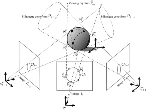
Figure 2.1: Shape from Silhouette approach: Three views with camera centre!cw i ,!cw(i−1)
and !cw
(i+1) produce silhouette cones and intersections (e.g., !pw1, p!w2, !pw3, !pw4, and p!w5)
approximate the volume of an object. Dotted lines on the object denote each contour generator and frontier points are marked as triangle, circle and square.
positions in front of the camera centres for illustration purpose. In the image plane Ii,
the occluding contourOiis extracted from the boundary of an object silhouette, i.e.,
Oi={!bi1,!bi2,· · ·,!bmi |dE(!bik,!bik+1)≤ √
2, 0≤k < m}, (2.1)
where dE(·) denotes Euclidean distance of two points and!bi is a point on the external
boundary of the silhouette, so thatOi defines a closed contour from a set of 8-connected
neighbour points. A silhouette cone whose apex is a camera centre, is then constructed
from a set of rays as illustrated by dotted lines in Figure 2.1 and points on an object that
touches a silhouette cone define a contour generator (see dotted curves on the object).
this convex region becomes a VH of an object, i.e,
VH =!
i=1
cone(Oi, Pi), (2.2)
where cone(·) is a function that constructs a silhouette cone by back-projecting an
oc-cluding contour using a projection matrixPi. Thus, a polygonal region defined by !pw1,
! pw
2,!pw3,p!w4 and!pw5 approximate the sphere shown in Figure 2.1. However, self-occluded
parts (e.g., small components behind the sphere) cannot be reconstructed correctly in
this view configuration and some concave regions which cannot be differentiable in the
image plane (e.g, inside of a mug) are reconstructed as convex.
Thus, one of the major concerns in early SfS is how to efficiently estimate the
intersection points of visual cones, and approaches regarding this problem are broadly
divided into two groups in terms of the space in which the intersection test takes place.
For example, with an approach of the first group, a 3D object is reconstructed by
back-projecting its 2D silhouettes (generated from different views) onto the 3D space, i.e.,
intersection test is performed in a 3D space. On the contrary, an approach belonging
to the second group projects approximately known 3D object positions onto the images
and carves the shape if the projections lie outside the corresponding silhouettes, i.e., the
intersection test is performed in a 2D space. Since the complexity exponentially increases
as the dimension of space increases, the approaches in the latter group are normally
preferred in recent SfS techniques. The other advantage of the 2D intersection test is
that it can integrate an octree structure easily into SfS for organising voxels.
Another important geometric entity is defined at the intersections of contour
gen-erators. In general, it is difficult to establish point correspondences solely based on two
occluding contours, because the shape of a silhouette is dependent on the viewing
di-rection. However, intersections of contour generators can give significant clue for the
boundary matching, and they are called frontier points, denoted by•,"and#in Figure
2.1. The methods shown in [15, 19] proposes VH construction by means of this
2.3
Visual hull representation
2.3.1
Octree representation
In computer graphics, surface models are generally represented by lists of vertices, edges
and faces, which are efficient in terms of rendering complex surface model, but it is not the
best representation for describing the volume of an object. Instead, the general volume
representation utilises various types of solid primitives (e.g., polyhedron, cylinder and
sphere) to describe an object by the combinations of these primitives. This volume
rep-resentation was widely utilised in early Computer Aided Design (CAD), which required a
suitable 3D model for the low level of graphical display [10]. As a combination method of
volume primitives, the Boundary Representation (B-Rep) describes the volume by surface
patches and their connection graph. The other method called Constructive Solid
Geom-etry (CSG) relates volume primitives using a tree structure of operation [20]. However,
B-Rep and CSG has limits when modelling arbitrary shape of an object. Furthermore, it
is not easily incorporated in SfS techniques.
An octree is a hierarchical tree structure of voxels and one octree is sufficient to
represent the volume of an object. Each node of an octree can have eight child nodes,
and the size of each dimension of a child node is half of the size of its parent node.
Therefore, the volume resolution of a VH becomes two times finer whenever the current
node produces offspring. To incorporate this structure into SfS, an initial bounding voxel,
i.e., an octant, should have sufficient volume to include an object, and an octant then
produces child nodes (i.e., split into 8 smaller octants) if a current octant intersects (or
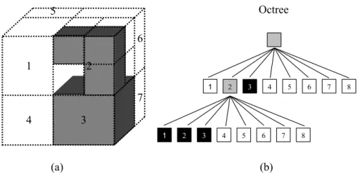
includes) an object until a tree meets the predefined level. For example, Figure 2.2(b)
illustrates a three-level octree formed from a simple object shaded as grey in Figure
2.2(a), where dotted cubes indicate nodes of an octree. The indices of the second level of
an octree are shown in both figures (a) and (b) for a direct comparison of a node in the
tree with its corresponding position in the 3D space.
Every node in an octree has a status, i.e., intersection, inside or background,
which indicates the result of an intersection test. The white, grey, and black rectangles in
Figure 2.2(b) respectively denote the background, intersection, and inside octants. Thus,
Figure 2.2: Example of an octree: (a) Grey voxels indicates the actual shape of an object, whilst dotted cubes represent the shape of octants. The indices correspond to the node indices in the second level of octree in (b); (b) A three-level of an octree of the object shown in (a), where black, white and grey node represent inside, background and intersection octant, respectively.
Classified as intersection, the octant is split into eight sub-octants to describe the object
in more details until the level of an octree reaches the predefined level. An initial voxel
enclosing an object is pre-determined manually, i.e., the root octant is the largest voxel
that consists of eight child octants indexed from 1 to 8 in Figure 2.2(a), where the eighth
octants is occluded by the fourth octant. Since the initial octant in Figure 2.2(a) includes
a grey object (i.e., an intersection case), it is split and the intersection test is repeatedly
applied to these smaller octants. Since the second octant in the second level of an octree
is classified as an intersection octant while the third octant is an inside octant, only the
second node is split into eight child nodes. Thus, four octants describes the object, i.e.,
the first, second, and third octants in the last level of the octree, and the third octant in
the second level of the octree.
As explained in Section 2.2, the intersection test can be performed faster in the
image plane. Thus, eight corner points of each octant are projected onto every image plane
by a camera projection matrix. The projections of corners generate a six-sided polygon
in the image plane, but the shape is normally approximated by a rectangle or a square
before the intersection test to further expedite the process. An algorithm proposed in [21]
Table 2.1: Octree updating rule.
Previous\ Current Unknown Background Intersection Inside
Unknown Unknown Background Intersection Inside
Background Background Background Background Background
Intersection Intersection Background Intersection Intersection
Inside Inside Background Intersection Inside
For example, each projected cube is converted into a bounding square and the status of
the bounding square is determined by single lookup of two distance maps constructed
from silhouette and its complement [21].
When an additional image is supplied, it is used to update the previous status
of an octant by constructing a new silhouette cone. The updating rule is summarised in
Table 2.1, where the status of a current octant estimated by a new silhouette image is
shown in the first row of the table and the previous statuses are presented in the first
column. As shown, the background status has top priority, i.e., it overrides other statuses.
The priority of other statuses is ordered as intersection > inside > unknown, which is
only required when describing the status of an initial octant. Alternatively, an octree
can also be constructed by the quadtrees of silhouettes, which traverses a tree structure
more efficiently than the traditional octree algorithm. However, three quadtrees from the
orthogonal directions are required to represent one object. Also, the projection method
is restricted as orthogonal transform [22], which is only satisfied when a camera is placed
in a distance from an object.
2.3.2
Silhouette detection
The SfS requires accurate silhouettes of an object for the intersection test, but it is a
chal-lenging task to devise an universal algorithm which adaptively processes an image for a
silhouette detection regardless of image conditions. Although there are some methods to
extract an object boundary from cluttered scene using an active contour [23], most
algo-rithms belonging to this category are based on iterative computation from many manually
selected thresholds with a good initial guess. Also, the result is not reliable in the presence
of large amount of clutter in the background, non-homogeneous texture of an object and
a preprocessing procedure in the whole reconstruction system, so that it needs to be
com-putationally simple (e.g., using intensity thresholding) but should retain a certain level of
robustness. Assuming a controlled scene (i.e., an object to be reconstructed is placed in a
homogeneous background under controlled lighting condition), some fundamental image
processing techniques such as Gaussian blurring, contrast enhancement and histogram
equalising, are selectively applied to an input image to improve the performance of the
silhouette detection by intensity thresholding.
However, this approach may include an artefact inside an object because of the
object texture having similar colour to background or shading produced by self-occlusion.
To address this problem, an occluding contour filled with the maximum intensity values
is used to represent a silhouette. Suppose that I#
i is a thresholded image from the i-th
imageIi, i.e.,
Ii#(!pik) =
1 ifIi(!pik)≥τint
0 otherwise
, (2.3)
where τint denotes an intensity threshold. In practice, Ii# may contain more than one
segment, which is the aggregation of connected nonzero points, even thoughIiis grabbed
from a controlled scene and enhanced with some image processing techniques. Assuming
there is only one object inIi, an occluding contour of an object is selected by a set of
connected boundary points with the maximum length in the image plane, i.e.,
Oi= arg max
k (|Ok|), (2.4)
where| · |indicates the cardinality of a set. Thus, a silhouette is produced by filling inside
the closed boundary setOi to produce a silhouetteSi in thei-th image. If inside cavities
of an object (e.g., handle of a mug) are taken into consideration in the reconstruction, the
internal boundaries of the largest segment are also utilised to accomplish the silhouette
detection, i.e., a set of internal boundaries is
Oint={
&
k
Ok |Ok∈ Si}. (2.5)
1 I p l I m a g e∗CImgProc : :
G e t S i z e F i l t e r I m g ( I p l I m a g e∗ imgBW, i n t nI ntC on )
3 {
/ / / / / / / / / / / / / / / / / / / / / / / / / / / / / / / / / / / / / / / / /
5 / / i n i t i a l i s e a r e t u r n b u f f e r
/ / / / / / / / / / / / / / / / / / / / / / / / / / / / / / / / / / / / / / / / /
7 I p l I m a g e∗ i m gRes = NULL ;
i m gRes = c v C r e a t e I m a g e ( c v G e t S i z e (imgBW) , 8 , 1 ) ; 9 i f (imgBW−>n C h a n n e l s > 1 ) r e t u r n i m gRes ; 11 / / / / / / / / / / / / / / / / / / / / / / / / / / / / / / / / / / / / / / / / /
/ / c r e a t e m e m o r y s t o r a g e
13 / / / / / / / / / / / / / / / / / / / / / / / / / / / / / / / / / / / / / / / / /
CvMemStorage∗ s t o r a g e = cv C reateMe m S t or a g e ( 0 ) ; 15 CvSeq∗ c o n t o u r = NULL ;
C v C ontourScan ne r s c a n n e r ;
17 s c a n n e r = c v S t a r t F i n d C o n t o u r s (imgBW, s t o r a g e ,s i z e o f( CvContour ) , CV RETR CCOMP, CV CHAIN APPROX NONE) ;
c o n t o u r = c v F i n d N e x t C o n t o u r ( s c a n n e r ) ; 19
/ / / / / / / / / / / / / / / / / / / / / / / / / / / / / / / / / / / / / / / / /
21 / / d e f i n e c o n t o u r s t r u c t u r e
/ / / / / / / / / / / / / / / / / / / / / / / / / / / / / / / / / / / / / / / / /
23 s t r u c t S C o n t o u r s
{
25 v e c t o r<C v Poi nt>∗ p a r C o n t o u r ;
i n t nTotCon ; 27 i n t n L o n g e s t C o n I d x ;
i n t nMaxLength ;
29 };
31 / / / / / / / / / / / / / / / / / / / / / / / / / / / / / / / / / / / / / / / / / / / i n i t i a l i s i n g
33 / / / / / / / / / / / / / / / / / / / / / / / / / / / / / / / / / / / / / / / / /
S C o n t o u r s a l l C o n t o u r s ; 35 a l l C o n t o u r s . nTotCon = 0 ;
a l l C o n t o u r s . n L o n g e s t C o n I d x = −1; 37 a l l C o n t o u r s . nMaxLength = −1;
Figure 2.3: Size filtering code snippet 1.
in the image plane is selected as an occluding contour, the seed-flooding algorithm [24]
follows to fill the inside of the contour to construct an initial silhouette. If internal holes
are further needed, internal contours are overlaid to the previously obtained silhouette,
and filled with the lowest intensity values. Since this method requires to sort all contours
in terms of their length, it is possible to filter (i.e., remove) small contours and selectively
include internal contours. Thus, this silhouette detection and filtering process is called a
size filtering in this thesis.
An image processing class CImgProc is designed to accomplish this goal. It
includes algorithms from simple image processing functions to the size filtering, which
have been developed mostly based on the Intel OpenCV library [25]. For example, the
function GetSizeFilterImg(·), as shown in Figure 2.3, is called with two input parameters,
e.g., a pointer of an initial thresholded image and the number of internal contours required.
Thus, if a variable nIntCon in line 1 is set to zero, the function returns a silhouette image
estimated only from an external object boundary. Lines from 7 to 9 create a memory
buffer that stores the resulting silhouette image, initialised as a 8-bit grey image with the
1 / / / / / / / / / / / / / / / / / / / / / / / / / / / / / / / / / / / / / / / / / / / a l l o w i n g i n s i d e c a v i t i e s
3 / / / / / / / / / / / / / / / / / / / / / / / / / / / / / / / / / / / / / / / / /
i f ( nI ntC on> 0 )
5 {
/ / / / / / / / / / / / / / / / / / / / / / / / / / / / / / / / / / / / / / / / /
7 / / 1 . h i t t e s t a n d r e m o v e t h e c o n t o u r s o u t s i d e a n o b j e c t / / / / / / / / / / / / / / / / / / / / / / / / / / / / / / / / / / / / / / / / /
9 v e c t o r<i n t> a r I n s i d e C o n t o u r I d x ;
f o r (i n t i = 0 ; i < a l l C o n t o u r s . nTotCon ; i++ )
11 {
i f ( i == a l l C o n t o u r s . n L o n g e s t C o n I d x ) c on t i n u e; 13 b ool b I s I n s i d e = t r u e;
f o r (i n t j = 0 ; j < a l l C o n t o u r s . p a r C o n t o u r [ i ] . s i z e ( ) ; j ++)
15 {
C v Poi nt2D 32f p t ;
17 p t . x = a l l C o n t o u r s . p a r C o n t o u r [ i ] . a t ( j ) . x ; p t . y = a l l C o n t o u r s . p a r C o n t o u r [ i ] . a t ( j ) . y ; 19 i f ( c v P o i n t P o l y g o n T e s t ( c o n t o u r , pt , 0 ) < 0 )
{
21 b I s I n s i d e = f a l s e;
break;
23 }
}
25 i f ( b I s I n s i d e )
a r I n s i d e C o n t o u r I d x . p u s h b a c k ( i ) ;
27 }
29 / / / / / / / / / / / / / / / / / / / / / / / / / / / / / / / / / / / / / / / / / / / 2 . o r d e r i n g
31 / / / / / / / / / / / / / / / / / / / / / / / / / / / / / / / / / / / / / / / / /
f o r(i n t i = 0 ; i < a r I n s i d e C o n t o u r I d x . s i z e ( ) ; i ++)
33 {
f o r(i n t j = 1 ; j < a r I n s i d e C o n t o u r I d x . s i z e ( ) − i ; j ++)
35 {
i f ( i n t ( a l l C o n t o u r s . p a r C o n t o u r [ i n t ( a r I n s i d e C o n t o u r I d x [ j ] ) ] . s i z e ( ) ) >
37 i n t ( a l l C o n t o u r s . p a r C o n t o u r [ i n t( a r I n s i d e C o n t o u r I d x [ j−1 ] ) ] . s i z e ( ) ) )
{
39 i n t nTemp ;
nTemp = a r I n s i d e C o n t o u r I d x [ j ] ;
41 a r I n s i d e C o n t o u r I d x [ j ] = a r I n s i d e C o n t o u r I d x [ ( j−1) ] ; a r I n s i d e C o n t o u r I d x [ ( j−1) ] = nTemp ;
43 }
}
45 }
47 / / / / / / / / / / / / / / / / / / / / / / / / / / / / / / / / / / / / / / / / / / / 3 . d r a w b l a c k i n t e r n a l c o n t o u r s
49 / / / / / / / / / / / / / / / / / / / / / / / / / / / / / / / / / / / / / / / / /
i f ( nI ntC on > a r I n s i d e C o n t o u r I d x . s i z e ( ) ) 51 nI ntC on = a r I n s i d e C o n t o u r I d x . s i z e ( ) ;
53 f o r(i n t i = 0 ; i < nI ntC on ; i ++)
{
55 cv EndFi ndC ont o u rs ( &s c a n n e r ) ;
s c a n n e r = c v S t a r t F i n d C o n t o u r s (imgBW, s t o r a g e ,s i z e o f( CvContour ) , CV RETR CCOMP, CV CHAIN APPROX NONE) ;
57 c o n t o u r = c v F i n d N e x t C o n t o u r ( s c a n n e r ) ;
f o r (i n t j = 0 ; j < a r I n s i d e C o n t o u r I d x [ i ] ; j ++) 59 c o n t o u r = c v F i n d N e x t C o n t o u r ( s c a n n e r ) ;
C v S c a l a r c o l o r = CV RGB ( 0 , 0 , 0 ) ;
61 cv D raw C ontours ( imgRes , c o n t o u r , c o l o r , c o l o r , 1 , CV FILLED , 8 ) ;
}
63 }
Figure 2.4: Size filtering code snippet 2.
that creates a stack memory structure to enclose a dynamic memory buffer (e.g., a linked
list).
The contour searching process in line 18 is provided by a function of OpenCV
(i.e., the process is optimised to an Intel processor2) and it returns the boundary of
an image segment as a pointer to a linked list, CvSeq*. Before calling the function
cvFindNextContour(·), it is required to initialise the contour retrieving properties (see
line 17). One can directly use a CvSeq pointer whenever it is needed, but all contour
2
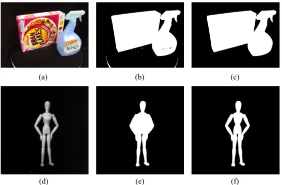
Figure 2.5: Example of silhouette detection: (a) objects with non-homogeneous texture; (b) thresholding result of (a); (c) a silhouette is estimated by applying the flood-seeding algorithm to the largest occluding contour; (d) an object with homogeneous texture but two internal cavities; (e) two inside holes cannot be distinguishable after the food-seeding algorithm; (f) two internal segments complete the silhouette detection.
data are temporarily organised in a user-defined local structure SContours (see lines 23
to 29) to facilitate data access. Thus, a variable, allContours defined in line 34, includes a
pointer of a vector data type3for storing all contours. Additionally, other useful variables
are temporarily stored, e.g., the longest contour index (i.e., an occluding contour), the
total number of segments in an image plane, and the length of the occluding contour.
Internal contours are used to create inside holes on an initial silhouette as many
as the input parameter (i.e., nIntCon) indicates. This process comprises of three steps:
searching internal contours, ordering internal contours with respect to their length, and
painting the inside of a hole with the lowest intensity values. More details of these
processes are shown in Figure 2.4, which is a part of the function GetSizeFilterImg(·) in
Figure 2.3. A variable arInsideContourIdx in line 9 stores all indices of internal contours,
determined by a hit test shown from lines 9 to 27. The bubble sorting estimates the
influence of an internal contour, i.e., the longer contour is the more influential it is. The
3
worst case complexity of the sorting algorithm isO(n2) [27], but the processing time in
practical applications is acceptable because the number of segments in an image is not
significantly large in a controlled scene. Finally, a function cvDrawContours(·) in line 61
paints inside of internal contours.
Figure 2.5 shows some results of the silhouette detection using the size filtering
algorithm. When an image does not have homogeneous texture, it is likely to have small
inside artefacts after thresholding. For example, an image shown in Figure 2.5(a) has
two objects (e.g., a cornflake box and a spray), and there are low intensity regions in the
object area (e.g., the label of the spray). In addition, Salt and pepper noise may appear
in a colour image sensor without Gaussian blurring [see the white dots in the turntable
area in Figure 2.5(b)]. Also, some bright regions outside an object can be presented in
an initial thresholded image [see the rim of the turntable at the bottom of Figure 2.5(b)].
The largest occluding contour with white filling excludes them in a silhouette image. As
a result, the algorithm generates a clean silhouettes as shown in Figure 2.5(c). On the
other hand, when an object has homogeneous texture but includes inside cavities, internal
boundaries are required to complete the silhouette detection. In Figure 2.5(d) the two
arms of a dummy produce two holes, which disappear if the largest occluding contour
is only used [see Figure 2.5(e)]. However, more details are retained after allowing two
internal contours as shown in Figure 2.5(f).
2.3.3
Octree construction
Two classes, one for describing a node of an octree named COctant and the other for
establishing an actual tree using COctant variables, are key classes for the C++
imple-mentation of octree construction. Private member variables of an octant class are listed
in Figure 2.6, where four integer values from -1 to 2 are also assigned to constant
vari-ables4 representing intersection results (line 4-7). Thus, a member variable m nStatus,
which indicates the status of an octant, only have one of these constants. To enhance
code reusability, the class is designed to also include colour information associated with
the corners of an octant (see line 26) in addition to their 3D corner positions (i.e., 24
double buffers are assigned for colour information of eight vertices in line 24). Also, it
4
1 / / / / / / / / / / / / / / / / / / / / / / / / / / / / / / / / / / / / / / / / / / / s t a t u s c o n s t a n t
3 / / / / / / / / / / / / / / / / / / / / / / / / / / / / / / / / / / / / / / / / /
#d e f i n e BACKGROUND 0 5 #d e f i n e OBJECT 1
#d e f i n e INTERSECTION 2 7 #d e f i n e UNKNOWN−1 9 #i n c l u d e<OpenCV/OpenCV . h>
11 c l a s s COctant
{
13 p u b l i c:
/ / / / / / / / / / / / / / / / / / / / / / / / / / / / / / / / / / / / / / / / /
15 / / c o n s t r u c t o r s a n d d e s t r u c t o r & / / o t h e r i n t e r f a c e f u n c t i o n s
17 / / / / / / / / / / / / / / / / / / / / / / / / / / / / / / / / / / / / / / / / /
. . . 19
p r ot e c t e d:
21 / / / / / / / / / / / / / / / / / / / / / / / / / / / / / / / / / / / / / / / / / / / m e m b e r v a r i a b l e s
23 / / / / / / / / / / / / / / / / / / / / / / / / / / / / / / / / / / / / / / / / /
C v Poi nt3D 32f m pts 3D V erte x [ 8 ] ;
25 / / e a c h s c a l a r h a s c o l o u r i n BGR o r d e r a n d t h e l a s t v a l u e i s v o t e
C v S c a l a r m s c C o l o u r [ 8 ] ; 27 f l o a t m f S i z e O f C u b e ;
i n t m n S t a t u s ; 29 COctant∗ m p o c t P a r e n t ;
COctant∗ m p o c t C h i l d r e n [ 8 ] ; 31 b ool m b N e e d T o D e l e t e I t ;
}
Figure 2.6: COctant declaration snippet 3
includes memory addresses of parent and children octants in m poctParent (line 29) and
m poctChildren (line 30), respectively, which enable a octree class to traverse nodes. A
boolean variable defined in line 31 indicates whether this octant needs to be destroyed in
an octree in accordance with the background status after a status update.
COctant is extensively utilised in COctree, which defines functions that arrange
node memory and update tree information. The class stores an octree in a matrix with
variable column length for the memory efficiency, i.e., thei−th row vector in the octree
matrix represents thei−th level of octree and the number of column elements is dependent
on the population in the generation. An octree is a similar to a family tree. For example,
octants in the same level of octree forms a generation, so that nodes in the row vector of the
octree matrix are also called siblings. If a node is deceased, all descendants produced from
the node no longer exist, i.e., a node cannot be inserted in the middle of a tree without
an ancestor. One restriction on an octree is that a node always produces eight children.
Thus, the maximum population of thei-th generation is 8(i−1), which means in the worst
casemgeneration of an octree requires'm
i=18(i−1)octants, and this exponential growth
of nodes makes an octree implementation slow and memory-intensive process. Therefore,
when the rectangular memory structure is used, it is easy to implement but only few cells
1 . c r e a t e C O ctree i n s t a n c e
2 / / a t t h i s s t a g e t h e r e i s n o c h i l d r e n b u t o n l y t h e f a m i l y f o u n d e r e x i s t s
2 . make f u l l f a m i l y member i n t h e l a s t g e n e r a t i o n , i . e . , 8 ˆ{( j−1)} o c t a n t s 4
f o r i = 0 u n t i l t h e end o f i m a g e s
6 f o r k = 0 u n t i l end o f o c t a n t s i n t h e l a s t g e n e r a t i o n 3 . p r o j e c t t h e k−t h o c t a n t o n t o t h e i−t h i m age
8 4 . d e c i d e t h e s t a t u s o f an o c t a n t
/ / i . e . , t h e c o m p l e x s t a t u s u p d a t i n g r u l e i s u n n e c e s s a r y
10 end f o r
e r a s e a l l b a c k g r o u n d o c t a n t s 12 end f o r
Figure 2.7: Octree construction method I snippet 4.
is designed to allow the variable length of a row vector, which is realised by adopting a
liked list structure to store siblings. For example, an array of pointers of sub-octants in
the same generation is stored as a linked list of COctant*, and multiple arrays from all
levels of the tree forms the octree matrix.
Two algorithms are implemented for the construction of an octree incorporating
the intersection test. A pseudo code shown in Figure 2.7 is designed to only exploit
octants in the last generation. If the last level of an octree is known, it is able to estimate
the total number of octants in the worst case. Therefore, two iterations [i.e., per view
iteration (see line 5 in Figure 2.7) and per octant iteration in the last generation (see line
6) in Figure 2.7] are sufficient to construct an octree, and the worst case complexity of
the algorithm isi×exp(j) (i.e.,i×8j), whereiandj represent the number of silhouettes
and the last level of an octree. It is an advantage of this method that iterations for
the progressive tree construction is not involved, i.e., functions for making offspring or
destroying descendants are not called inside the iteration. However, the initial octree
construction from the first two views takes most of construction time if the level of an
octree is high because all octants in the last generations are unnecessarily projected for
the intersection test. Furthermore, the resolution of a simple shape is unnecessarily high
because the a VH only uses the finest resolution of an octant, which consequently increases
the size of final 3D data.
The second algorithm shown in Figure 2.8 is more memory efficient and faster than
method I, if the shape of an object is not significantly complex. The octree construction
method II consists of three major processes: initialising an octree (line 1), projecting an
octant (line 7), and updating status of a node (line 9), which are incorporated in triple