Multi band protocol accuracy

Victor Goossens 7/5/2015

2

Summary

With diffusion magnetic resonance imaging (MRI) imaging the elapsed time of the scan can be cut in half or even less if more than one slice is simultaneously acquired. This way more diffusion directions per minute can be obtained. In this project several protocols with varying multi-bands and directions are analyzed for their accuracy. The MB3 (multi-band 3) protocol was a lot less accurate than the MB1 protocol although the amount of directions was about one and a half times as big as the MB1 protocol. It was especially bad at the core of the brain. The MB2 protocol showed that in the same elapsed time as the MB1 protocol, the accuracy at the outside of the brain was increased. This was because of the double amount of used directions in the same elapsed time. The core of the brain of the MB2 protocol was still worse, while overall it was the same accuracy.

Introduction

The MRI scan technique is a powerful and flexible tool to analyze the brain. It uses the signal attenuation caused by water diffusion in the brain to locate the white matter in the brain. Diffusion tensor imaging (DTI) uses the information from the scan to create a characterization of the three-dimensional diffusion of the water in the brain as a function of the spatial location. It gives a diffusion tensor for every location in the brain which describes the magnitude, degree of anisotropy and the orientation of the diffusion anisotropy. It can then use the diffusion anisotropy and the principal diffusion direction to estimate the axon patterns.

DTI methods keep evolving and with them the accuracy of the methods. They have greatly improved over the years and further improvements are expected. New pulse sequences are continuously being developed to improve the spatial resolution and the accuracy and decrease artifacts in DTI. All these new protocols need to be analyzed for their accuracy.

In this project, ways to work with the data from the MRI-scans and different methods to make masks to focus on the white matter data from a scan will be shown, DTI will be discussed and a method to tell the accuracy of certain protocols will be developed and will be used to analyze different multi-band

protocols.[1]

Goal

Finding the qualitative and quantitative differences between different DWI scan protocols.

Hypothesis

3

Theory

In this section the basics for DTI and a useful technique to help with the analyzing of white matter are discussed.

Diffusion

Diffusion is a random transport phenomenon of material transfer from one location to another over time. The formula for diffusion is called the “Einstein equation” and looks like this:

= ∆_∆ (1)

The diffusion coefficient, D, is proportional to the mean squared-displacement divided by number of dimensions, n, and the time, Δt. This random transport of material is in water mainly caused by random thermal fluctuations. The diffusion of water in tissue gets influenced by cellular membranes and organelles. In a big body of water the diffusion will be the same in all directions, but in the

neighbourhood of cellular membranes it will diffuse more in the direction of the axons. This is because the cellular membranes hinder diffusion. In the brain’s white matter the tissue is fibrous and the diffusion in the direction parallel to the axons is relatively high compared to directions perpendicular to the axons. So the diffusion in white matter is, in contrast to the rest of the brain (grey matter and the cerebrospinal fluid (CSF)), anisotropic.

DWI

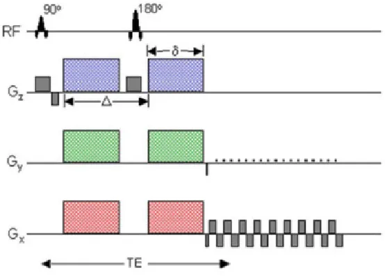
Diffusion-weighted imaging (DWI) is a MRI scan technique that measures the diffusion in the brain. The most common DWI approach is the pulsed-gradient, spin echo (PGSE) pulse sequence with a single-shot, echo planar imaging (EPI) readout. This approach is shown in Figure 1.

4 First a gradient pulse is send through the brain, which linearly dephases the magnetization in the voxels in the direction of the gradient, which is a combination of a gradient in the x, y and z direction. After a 180 degrees refocusing pulse, a second reversed gradient pulse is used. If a particle has not moved, the two pulses will completely cancel for that particle. If that is the case for all the particles at that voxel it will send a strong signal because they are all in phase. If particles have moved in the direction of the applied gradient, the two pulses will not cancel each other. This will cause the sent signal to become weaker because of destructive interference. This signal loss is described by the formula:

= exp (−( (∆ − ) (2)

Here S is the signal strength, the signal without gradient pulses (but otherwise same parameters), the gyromagnetic ratio, the duration of the pulse, G the strength of the pulse, ∆ the time between the pulses and D the diffusion coefficient. Another way to write this formula is:

= exp (−b ) (3)

Now b is the factor that can be adjusted at the beginning of the measurement by changing the shape of the pulse and duration between pulses. It is called the b-value. The other parameters are the unknown variables.

To be able to determine the unknown variables in Formula 3 a certain amount of measurements must be made. One measurement must be made to determine the S0 factor and at least 6 more to determine the whole diffusion tensor.

DTI

A way to describe the diffusion in the brain is with the help of a diffusion tensor. This tensor is a 3x3 covariance matrix.

Figure 2: description of the isotropicy/anisotropicy with the eigenvalues tensor

With the three lambda’s some properties of the diffusion can be represented with analyzing the data. The mean diffusio

degree of diffusion. Another useful parameter is the fractional anisotropy (FA). = ( ! "(_" ! "(_"

The FA describes how anisotropic the voxel is, with 0 being isotropic and 1 highly anisotropic. This factor is higher in white matter in comparison to the rest o

3 (left).

Also with the eigenvalues and the eigenvecto

The dyads describe the direction of the anisotropy and can be plotted in a red shows the direction of the diffusion in

dispersion of the dyads direction.

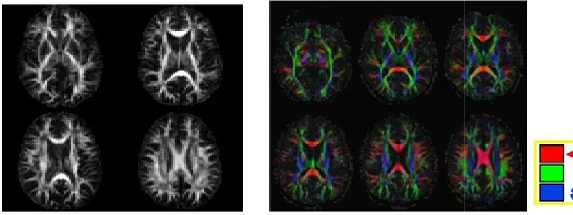
Figure 3: Image of the brain showing the FA (left) and the anisotropic direction (right) Figure 2: description of the isotropicy/anisotropicy with the eigenvalues and eige

lambda’s some properties of the diffusion can be represented, which could be helpful with analyzing the data. The mean diffusion (MD) is the mean of the three lambda

useful parameter is the fractional anisotropy (FA). ( !

w anisotropic the voxel is, with 0 being isotropic and 1 highly anisotropic. This factor in white matter in comparison to the rest of the brain and is very useful in locating it

ith the eigenvalues and the eigenvectors, the dyads and the dyads dispersion can be The dyads describe the direction of the anisotropy and can be plotted in a red-green

the direction of the diffusion in color, see Figure 3 (right). The dyads dispersion descr dispersion of the dyads direction.

Figure 3: Image of the brain showing the FA (left) and the anisotropic direction (right)

5 envectors of the diffusion

which could be helpful is the mean of the three lambdas and describes the

(5) w anisotropic the voxel is, with 0 being isotropic and 1 highly anisotropic. This factor

f the brain and is very useful in locating it, see Figure

the dyads and the dyads dispersion can be calculated. green-blue plot, which (right). The dyads dispersion describes the

6

Making a mask

When data from a scan are analyzed it is important the right data is analyzed. In this case the only data of interest are the white matter. To get the clearest results, the rest of the data (the grey matter and the CSF) should be ignored. This ignoring can be accomplished by multiplying the data with a matrix. That matrix multiplies the white matter by one and the rest of the data by zero. The matrix that multiplies the voxels by zero or one is called a mask.

The difference between white matter and the rest of the brain is the high anisotropy in the white matter. So to create a mask, a reference dataset should be used which describes the anisotropy. Next the cut-off value for white matter or not must be decided, if this value is too low there will be too much grey matter in the data, but if this value is too high there will be too much data loss.

Now the noise in the data must be filtered out. Because the noise comes mostly as high valued voxels, it can be filtered by comparing the data points with its neighbours. If not enough neighbourhood particles are also higher value voxels, the voxel will be cut off. When to cut off a certain voxel is important to decide. If not enough is cut off there will be a lot of noise and if too much is cut off there will be data loss.

Protocols

Every measurement, some parameters can be adjusted to increase or decrease the accuracy, elapsed time and resolution. An important parameter is the b-value. As discussed in the DWI section, it consists of more parameters, but the important factor is the final value of the b-value. If it is too low the distinction between high and low diffusion is harder to make, but if it is too high there will be too much signal decay. A usual value for brain tissue is around 1000. Another parameter is the resolution, higher resolution means higher accuracy but also more elapsed time. The same is true for the amount of directions used and the relaxation time. A factor that can greatly reduce the elapsed time is the multi-band factor. This factor describes how many slices are excited and measured simultaneously. By scanning two slices at the same time, the elapsed time will be halved. However, this technique will cause a severe reduction in accuracy called the g-factor penalty. Since the aliased slices are generally close to each other due to a comparatively small field of view (FOV) in the slice direction (e.g. FOVslice =12

cm vs. FOVinplane =21 cm). [3][4]

Measuring procedure

In this section the several steps taken in this project are discussed.

DWI scan

7

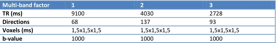
Multi-band factor 1 2 3

TR (ms) 9100 4030 2728

Directions 68 137 93

Voxels (ms) 1,5x1,5x1,5 1,5x1,5x1,5 1,5x1,5x1,5

b-value 1000 1000 1000

Table 1: Used protocols for the different multi-band factors.

The b-values and the resolution are the same for every protocol. The amount of directions of protocol MB2 is two times that of protocol MB2 so the total elapsed time will be the same for those protocols. The total elapsed time for the MB3 protocol is about the half of the other two protocols.

Data processing

After the scan there are separated datasets from all the measured direction. These datasets are put in a matlab program called DD_basicproc.m which gives as output, among other things, the FA, the AD and the b-values. If this data is put in another program called bedpostX it gives as output, among other things, the dyads and the dyads dispersion.

Matlab script

The used matlab script for this project is shown in the Appendix. In this section the steps of the script will be explained.

The input of the matlab function is the directory of the bedpostX output folder for both of the datasets. It then loads the FA dataset from the first directory and creates a mask with it by cutting off all voxels with a value less than 0.15. It then goes through three for-loops, with which it goes through all the voxels of the dataset and three for-loops within those to look at every neighbourhood voxel to determine how many more “white matter” is surrounding it. If that value is not enough it gets cut off. Afterwards it does the same for the other directory and multiplies the two masks so no dataset gets favored by the mask.

After the dyads dispersion of both directories is loaded, the data sets get multiplied by the mask and the average dispersion per white matter voxel is calculated. The overall quality of the protocol gets

8

Results

In this section the results of the project are shown.

Quantitative difference

As shown in Table 2 the quantitative difference between MB1 and MB2 is very small, while the difference of MB1/MB2 and MB3 is a lot bigger.

Dir1 \ Dir2 MB1 MB2 MB3

MB1 0 0.0013 -0.0359

MB2 -0.0013 0 -0.0352

MB3 0.0359 0.0352 0

Table 2: difference in dyads dispersion per voxel (In the left the protocol in the first directory input and in the top the protocol in the second directory input).

Qualitative difference

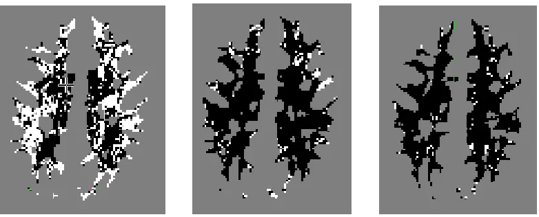
As shown in Figure 4, the MB1 protocol has at most voxels at the outside higher dyads dispersion in comparison with the MB2 protocol, while the MB2 protocol has more voxels with higher dispersion at the core. The same is the case when comparing MB1 and MB3, although in this case there are a lot more black voxels, so the dyads dispersion is for most voxels higher for MB3.

Figure 4: difference in dyads dispersion between protocols with white meaning the first protocol has higher dyads dispersion and black the second protocol has higher dyads dispersion. (left MB1 and MB2, middle MB1 and MB3 and right MB2 and MB3).

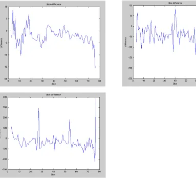
Slice difference

9

Figure 5: The slice differences of the protocols (left above MB1, right above MB2 and left under MB3)

Conclusion

When looking at the qualitative differences between the protocols in Figure 4, protocol MB1 is worse at the outside of the brain, but better at the core of the brain compared to the MB2 protocol. Protocol MB3 is just overall worse than the other two protocols, but compared to the MB1 protocol the core of the brain is especially bad.

When looking at the quantitative differences between the protocols in Table 2, MB3 is a lot worse than protocol MB1 and MB2, while MB1 and MB2 are not that different quantitatively.

10 The MB3 protocol had a lot less accuracy than both other protocols, both quantitative and qualitative, even though its amount of used directions is higher than the MB1 protocol. It must be noted that the used time for the MB3 protocol is halve of that of the other two protocols and it would probably increase the accuracy a lot if that was doubled.

There is not a real pattern to detect in the slice differences in Figure 5, for every second slice for the MB2 protocol or every third slice for the MB3 protocol. The larger differences at the top and the bottom slices of the brain can be explained by the lower amount of white matter. Because when there is a lower amount of samples the standard deviation will be larger.

Evaluation

It might have been better if the project was done with six protocols, where in the first three the elapsed time would stay the same with the change of multi-bands, but increased directions. In the second three, the directions would stay the same and the elapsed time would change with the change of multi-bands. This way the conclusion could be more certain about the cause of the increase or decrease in accuracy.

References

[1] A.L. Alexander, J.E. Lee, M. Lazar, A.S. Field, 2007. Diffusion tensor imaging of the brain. Neurotherapeutics 4(3), 316-329

[2] G. J. Barker, 2014. Diffusion goes mad.

11

Appendix

function procheck2(dir1,dir2)

%% Load data mask1 and slice difference 1

cd(dir1) cd .. dir3=[cd,'/FDT_Data/']; cd(dir3); fa1=ls('fa*'); fa1=strtok(fa1); fa1=load_untouch_nii(fa1); fa1.img=fa1.img(:,:,1:80); data_nii1=load_untouch_nii('data.nii.gz'); data1=data_nii1.img(:,:,1:80,1); data1=make_nii(data1); %% Mask1 [x,y,z]=size(fa1.img); f1mask1=fa1.img>0.2; f1mask1(:,:,1)=0; f1mask1(:,:,z)=0; for k=2:x-1 for l=2:y-1 for m=2:z-1 bl=0; if fa1.img(k,l,m)>0.2 for r=-1:1 for s=-1:1 for t=-1:1 if fa1.img(k+r,l+s,m+t)<0.2 bl=bl+1; end end end end if bl>5 f1mask1(k,l,m)=0; end end end end end f1mask1=+f1mask1;

%% Load data mask2

12 bl=0; if fa2.img(k,l,m)>0.2 for r=-1:1 for s=-1:1 for t=-1:1 if fa2.img(k+r,l+s,m+t)<0.2 bl=bl+1; end end end end if bl>5 f1mask2(k,l,m)=0; end end end end end f1mask2=+f1mask2;

%% f1 Mask

famask=f1mask1.*f1mask2;

%% Load data dispersion

cd(dir1); dyads_disp1=load_untouch_nii('dyads1_dispersion.nii.gz'); dyads_disp1.img=dyads_disp1.img(:,:,1:80,1); cd(dir2); dyads_disp2=load_untouch_nii('dyads1_dispersion.nii.gz'); dyads_disp2.img=dyads_disp2.img(:,:,1:80,1);

%% Average dispersion

masked_disp1=dyads_disp1.img.*famask; total_disp1=sum(masked_disp1(:)); total_mask1=sum(famask(:)); average_disp1=total_disp1/total_mask1; masked_disp2=dyads_disp2.img.*famask; total_disp2=sum(masked_disp2(:)); total_mask2=sum(famask(:)); average_disp2=total_disp2/total_mask2;

%% Difference dispersion

diff_disp=average_disp1-average_disp2 if diff_disp<0

'protocol 2 is overal worse' end

if diff_disp>0

'protocol 1 is overal worse' end

if diff_disp==0

'that is unlikely..., this might be the same data' end

%% Local dispersion difference

loc_disp_diff=(dyads_disp1.img-dyads_disp2.img).*famask; fv(loc_disp_diff)

%% take difference between slices

[~,~,s]=size(data1.img); if ((s/2)-floor(s/2))==0

13

datadiff1=data1.img(:,:,1:2:end-1)-data1.img(:,:,2:2:end); datadiff2=data1.img(:,:,2:2:end)-data1.img(:,:,3:2:end); end

%% mask all the pixels that are not white matter in the two slices

if ((s/2)-floor(s/2))==0 datadiff1=datadiff1.*(famask(:,:,2:2:end).*famask(:,:,1:2:end)); datadiff2=datadiff2.*(famask(:,:,2:2:end-1).*famask(:,:,3:2:end)); else datadiff1=double(datadiff1).*(famask(:,:,2:2:end).*famask(:,:,1:2:end-1)); datadiff2=double(datadiff2).*(famask(:,:,2:2:end).*famask(:,:,3:2:end)); end

%% total difference per slice

[~,~,k]=size(datadiff1); for i=1:k datadiff11=datadiff1(:,:,i); dataslicediff1(i)=sum(datadiff11(:)); total_mask11=famask(:,:,2*i).*famask(:,:,2*i-1); total_mask1(i)=sum(sum(total_mask11(:))); faslicediff(i*2-1)=dataslicediff1(i)/total_mask1(i); end [~,~,l]=size(datadiff2); for j=1:l datadiff21=datadiff2(:,:,j); dataslicediff2(j)=sum(datadiff21(:)); total_mask21=famask(:,:,2*j).*famask(:,:,2*j+1); total_mask2(j)=sum(sum(total_mask21(:))); faslicediff(j*2)=dataslicediff2(j)/total_mask2(j); end figure plot(1:(l+k),faslicediff)

%% take difference between slices

[~,~,s]=size(data2.img); if ((s/2)-floor(s/2))==0 datadiff1=data2.img(:,:,1:2:end)-data2.img(:,:,2:2:end); datadiff2=data2.img(:,:,2:2:end-1)-data2.img(:,:,3:2:end); else datadiff1=data2.img(:,:,1:2:end-1)-data2.img(:,:,2:2:end); datadiff2=data2.img(:,:,2:2:end)-data2.img(:,:,3:2:end); end

%% mask all the pixels that are not white matter in the two slices

if ((s/2)-floor(s/2))==0 datadiff1=datadiff1.*(famask(:,:,2:2:end).*famask(:,:,1:2:end)); datadiff2=datadiff2.*(famask(:,:,2:2:end-1).*famask(:,:,3:2:end)); else datadiff1=datadiff1.*(famask(:,:,2:2:end).*famask(:,:,1:2:end-1)); datadiff2=datadiff2.*(famask(:,:,2:2:end).*famask(:,:,3:2:end)); end

%% total difference per slice

14

total_mask2(j)=sum(sum(total_mask21(:)));

faslicediff(j*2)=dataslicediff2(j)/total_mask2(j); end

figure