Crossing Obstacles

(1)

Crossing Obstacles

Report of my training period at the department of flow control,

School of Aeronautics and Astronautics,

Zhejiang University, Hangzhou, China.

author: Cijsouw Wout

supervised by: MSc. Chen Ming

Dr. Lingxin Zhang

(2)

Chapter 1 Introduction

To everyone who is intended to read this report,

Since my training period at the Zhejiang University has come to an end, I hereby present my report. In this report I will try to give an overview of my achievements during this period.

The title of this report is partially based on the subject of the training period, which was cavitation at hydrofoils. Obstacles were attached to the hydrofoil to reduce the cavitational volume. Besides crossing obstacles in the experi-mental setup, there were a lot of obstacles to cross before my enrollment as a student at the Zhejiang University.

Before I start with describing all MATLAB scripts I have produced during this period, I would like to thank a view people who have been really important to me during this period.

First of all I would like to thank Dr. Lingxin Zhang who offered the possibility of having this training period at his department. Upon my arrival everything was well prepared and organized. During the department meetings Doctor Zhang gave me feedback and some advices. Furthermore a lot of opportunities were offered from his side, for instance to join in a conference organized for departments of flow control from different universities.

The research in which I participated is designed and performed by Chen Ming who I directly met upon my arrival in Shanghai. Ming showed me everything about the Zhejiang University, introduced me to his friends and helped me with all of the issues that emerged during all of the obstacle crossing. Above all, Ming learned me everything about life in China with a lot of humor. Since we were in close cooperation this was all really convenient.

I went to China without having any clue how to obtain the required student visa. Luckily Yueping Xu from the de-partment of water management at the Zhejiang University knew everything about the procedure to obtain the required documents. Yueping, thank you for your help!

During the training period there were many persons more who helped me with all of my issues. Especially everyone who was in my office and in the other office belonging to the department have helped me a lot, thank you all!

At last, I would like to thank professor Hoeijmakers at the University of Twente, who, somehow, achieved to arrange the right contacts for this training period. Furthermore, professor Hoeijmakers has always supported me in participating in this training period, even when it seemed very difficult to obtain the right documents.

(3)

Chapter 2 Cavitation on hydrofoils

2.1. Cavitation

If a liquid like water is subjected to a (temporarily) lowered pressure, the liquid will evaporate. No external heat source is required for evaporation if the pressure is below the vapor pressure. This process of evaporating caused by a lowered pressure is calledCavitation.

Cavitation in its most simple form causes vapor bubbles in the liquid. There are two more forms in which cavities (as a cavitating bubble, sheet or vortex is called) may appear: sheet cavities and cavitating vortices, as stated in ”Funda-mentals of Cavitation” [2]. Sheet cavities can be seen at for instance a hydrofoil or a turbine blade. The cavitating vortices can be seen in the low-pressure vortex core at for instance the tip of a foil.

Since cavitation is a phenomenon which occurs only in low pressure regions, the cavity, will collapse when the pressure increases. The cavities often collapse violently since the pressure differences between the internal bubble pressure and the local pressure are very large. The bubble collapses can for instance cause structural damages, reduce the efficiency or cause noise and vibrations to the object to which the cavity is attached.

2.2. Hydrofoils and cavitation

Cavitation occurs in many machines, varying from ship propellers to surgical tools. The research described in this report is regarding sheet cavitation on hydrofoils. In many marine applications hydrofoils are used to improve stability and/or achieve higher velocities, an example of an application is shown in figure 2.1(a). Since the hydrofoil attached to this boat (which is actually below the water surface) has a lower resistance compared to the hull of the boat, the maximum achievable speed of the boat will be higher when using the hydrofoil.

(a) Boat which uses a hydrofoil to achieve higher veloci-ties, source: www.seattlepi.com

(b) A hydrofoil and the pressure distribution

Figure 2.1

A schematic drawing of a hydrofoil can be seen in figure 2.1(b). In this figure the low pressure and high pressure regions around the foil are indicated. When sailing, cavitation on the low pressure (high velocity) side of the foil can occur. This will usually be due to combination of velocity, static pressure and the fluid vapor pressure. Cavitation will occur when thecavitation number, equation 2.1, is below a critical value.

σ= p₁−pv

2ρv

2 (2.1)

In this equationσis the cavitation number,pis the local pressure,pv(T) is the vapor pressure,ρis th density of the

liquid andv is the flow velocity.

2.3. Hydrofoils and cavity shedding

When the flow velocity of the 2D-hydrofoil in figure 2.1(b) reachesσcritical, a small sheet cavity will appear at the

(5)

a cloud cavity. This will usually happen in a periodic pattern, causing shedding of the cloud cavities. This periodic behavior can be really harmful to the hydrofoil.

To eliminate this shedding behavior, the mechanism of cloud forming and collapse are of interest.

• The mechanism that is probably most widely accepted is cavity pinch off at the leading edge of the cavity, by a re-entrant jet. Because of violently collapsing vapor bubbles at the trailing edge of a cavity, a water jet is formed at the trailing edge. This water jet will travel to the leading edge of the cavity in the low pressure region between the top side of the foil and the bottom of the cavity. At the leading edge, the sheet cavity is pinched off and a cloud cavity is formed. When this cloud cavity collapses, it will be responsible for the next re-entrant jet. In this way periodic behavior can be found. This mechanism is explained in more detail by the research of Kawanami et al. [4].

• Another proposed mechanism is cavity breakdown by condensation shock. A condensation shock travels from the end of the cavity up to the leading edge. Causing cavity pinch off at the leading edge. This mechanism was found by Harish Ganesh [3] using x-ray measurements.

(6)

Chapter 3 Cavity reduction on hydrofoils

3.1. Experimental setup

During the training period experiments were performed in the Zhejiang University cavitation tunnel. A hydrofoil with various obstacle configurations was studied. High speed images and the pressure signal of a hydrophone were collected to examine the cavity volume. Using MATLAB, the images of the high speed camera were processed to calculate the cavity volume.

3.1.1. Zhejiang University cavitation tunnel

The cavitation tunnel at the Zhejiang University is a closed loop cavitation tunnel (5.8mhigh, 5.2mwide) which has a test section area of 200x200x1000mm. A schematic drawing with a clear description of the tunnel can be seen in Appendix 8.2. A picture taken during operation can be found in figure 3.1(a). The tunnel’s axial pump is able to reach flow speeds up to 12m/s, and pressures as low as 0.2 atm can be achieved. The tunnel is equipped with a vacuum system to eliminate air, this vacuum system usually runs one day before performing experiments. The pressure before and after the converging duct in front of the test section is measured.

3.1.2. Hydrofoil

The hydrofoils that were used during the experiments can be seen in figure 3.1(b). The hydrofoils have a series of slots in which the obstacle are inserted. When no obstacle was required, a slot could be inserted with the height of the foil. After inserting the required slots, the foil received a paint job for surface smoothness. Both foils are 3D printed. Due to damage during installation the aluminum foil has never been used. After six series of experiments, the plastic foil started to bend downward, therefore the experiments were stopped and a new foil was ordered. A drawing of the foil and one obstacle can be found in figure 8.3 in the appendix.

(a) Test section during experiments (b) Plastic (left) and aluminum foil (right)

Figure 3.1

3.1.3. Camera’s and light

The camera’s used are a Photron Fastcam to record images from the top and a HX-3 MEMRECAM for recording images from the side. Both able to record images at 5000 frames per second. The trigger signal for the Camera’s and the hydrophone was was generated using an electrical pulse caused by a battery. The light sheets were created by three lamps with a variable focus and light intensity. The focus was spread as much as possible to create a convenient light sheet. The light intensity was reduced as much as possible to minimize reflections on the foil. The setup of the camera’s and lights can be seen in figure 3.1(a).

To prevent burglary of the highly expensive equipment, the camera’s were disassembled after each set of experiments. As a consequence, the camera’s had to be re-installed before every set of measurements. Resulting in different camera positions and zoom rates between experiments.

3.1.4. Hydrophone

(7)

Chapter 4 Matlab code for experiment analysis

In the field of cavitational flow experiments, PIV analysis and high speed image recordings are often used to investigate the flow phenomena. It is however hard to process the resulting images to data which is suitable for analysis. In the research performed by E.J.Foeth [1], commercial PIV software was used to visualize the flow of a 3D sheet cavity. In the research of Michael Wright [6], a MATLAB script was used to measure the propagation distance, cloud velocity and pulsation frequency of a cavitation cloud caused by a submerged water jet. These processing programs are however only suitable for 2-D image processing. As far as known to the author, only Harish Ganesh [3] used an algorithm which is suitable for the analysis of images of a 3D cavitating flow. This report became available to the author after the code described in this chapter was written.

Because there was no suitable software available for this kind of analysis, it was decided to develop a series of MATLAB scripts which can analyze the experimental data. The method used for this analysis will be discussed and explained in this chapter. In chapter 8.1 there is a short manual available for the one who is interested in using the MATLAB scripts.

4.1. Images resulting from the experiments and preprocessing

From both the side and top view, movies of 5000 frames (1 second) are extracted and saved. The movies are processed to .tiff (image)files using the Photron and HX Link software. The images resulting from the top view are horizontally mirrored to match the flow direction with the side view images. The side view (figure 4.1(a)) and top view (figure 4.1(b)) images, are not equally sized and zoom rates are different as well. Furthermore, zoom rates will vary between each set of experiments, because of daily break down (section 3.1.3). Therefore the MATLAB script has to be able to resize the images to obtain reliable results.

(a) Original image of the side view (b) Horizontally mirrored image of the top view

Figure 4.1

4.2. Required output and general principle for calculations

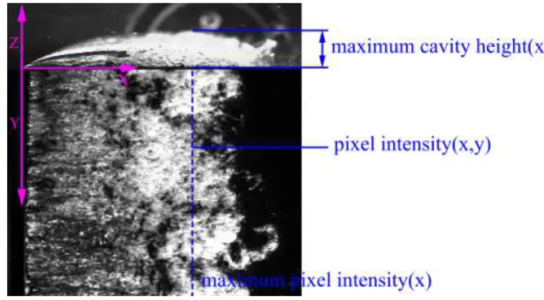
To find the most suitable obstacle location for volume reduction, the volume of the cavities is required. Therefore, the volume has to be calculated for each top and side view image pair. The method used to calculate the volume is based on linear relation equation 4.1.

cavity height(x, y) =pixel intensity(x, y)∗ maximum cavity height(x)

maximum pixel intensity(x) (4.1)

(8)

Figure 4.2: Locations of the obtained variables

4.3. Script 1: Determine foil and cavity location in the images.

The first script used for the analysis: ”BoundariesLocation.m” calculates the average of an user defined number of images. This average will result in an image which can be used to find the edges of the hydrofoil and the cavity inception locations.

4.3.1. Calculation of the averaged images

To start the analysis, MATLAB will require some user defined input. Thereater, all images are automatically loaded from their file locations. When loaded, a summation over all matrices is performed. The average is obtained by dividing this summation by the number of images used, liked stated in equation4.2.

Iaverage(xp, yq) =

1

n

X

i=1

Ii(xp, yq) (4.2)

In this equationIaverage(xp, yq) represents the averaged image of sizepxqpixels,nis the user defined number of images

andIi(xp, yq) are the individual images.

The result of this averaging step can be seen in figure 4.3(b). For calculating the average, every 8th image will be used by default (8 images will be skipped from the image folder). This is done to use the entire cavity dynamics for analysis, including all minimum and maximum cavity shapes.

(a) one single image of the side view (b) average of 20 images at the side view

Figure 4.3

4.3.2. Hydrofoil edges and cavity inception point

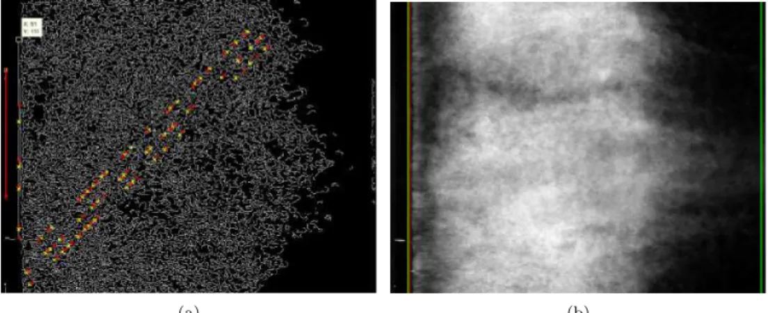
As soon as the average of the images is calculated, a MATLAB edge detection function is used to detect the edges present in the image. The results of this edge detection method, are represented by all white colored lines in in figure 4.4(a). The method used for this edge detection method, is the Canny edge method, since this method appeared to produce the least amount of noisy edges.

When the edges are detected, a hough transform is used to find the coordinates which are most likely to form an edge. For this, the algorithm uses a transformation from to cylindrical coordinate space. The hough transform that is used here will plot the 5 coordinate combinations which are most likely to form lines. This can be seen in figure 4.4(a). The results do not always give the desired output. Therefore, the user has to select the upper and lower edge manually.

(9)

(a) Side view contour plot after Hough transform (b) Side view after edge detection selection script

Figure 4.4

4.3.3. Gray level and cavity inception

When the user has supplied the desired edge locations, MATLAB will draw lines at the upper and lower edge of the foil. These lines can be used for visual inspection of the location of the lines. The edge locations will be used in later analysis to determine the scaling of the images. In this script, the cavity inception point, which is basically chosen as the first white pixel in a binary colored image is found as well. In figure 4.4(b), this is the red line.

The edges of the foil and the cavity inception point are saved automatically to be used for later analysis.

4.3.4. preprocessing the top view

The top view is preprocessed using the same edge selection procedure. The cavity inception point, leading and trailing edge of the foil are found. Not the tip of the foils wedge is used but the leading edge at the upper surface of the foil. In figure 4.5(a) it can be seen that MATLAB is not able to find the trailing edge of the foil. In this case, this trailing edge has to be selected manually.

(a) (b)

Figure 4.5: Edge detection and edge locations for the top view images

4.4. Script 2: averages

The next MATLAB script to be used is ”ImagesAverage.m”. This script calculates the average of a user defined number of images, in a similar way like in the previous script (section 4.3.1). Therefore the method of averaging is not discussed in detail.

It is however important to realize that the purpose of the second averaging step is for analysis efficiency. When using the currently available hardware and MATLAB knowledge of the author, MATLAB will run out of memory at about 300 images. By using every single image pair, only 0.06 seconds of cavity behavior can be calculated, which is sufficient to calculate only on or two shedding cycles. Therefore the average of everynimages is used to determine the volume.

n is defined by the user and is usually chosen between 4 and 6. The resulting images of the side view are shown in figure 4.6

(10)

Figure 4.6: one single image (left) and the average of 5 images (right) bubbles will be reduces by this averaging step.

Another advantage of this averaging step is that the resulting volume-time behavior will become more smoothly since the high cavity peaks are averaged of n images. The averaged images will be stored in a .mat file and can be used in the final script for the volume analysis.

4.5. Script 3: bubble volume

The last MATLAB script which makes use of the images themselves is ”BubbleVolume.m”. This script uses the averaged images from the previously discussed script to determine the cavity volume for every time step. According to equation 4.1, three variables are required to calculate the cavity height and therewith the volume.

• maximum cavity height(x), Which can be obtained from the binary colored side view.

• maximum pixel intensity(x), Which can be obtained along each x-coordinate in the top view.

• pixel intensity(x, y), Which can be obtained from each coordinate in the top view.

BubbleVolume.m is able to obtain these variables and to calculate the cavity volume using these variables.

4.5.1. Resize, rescale and recolor images

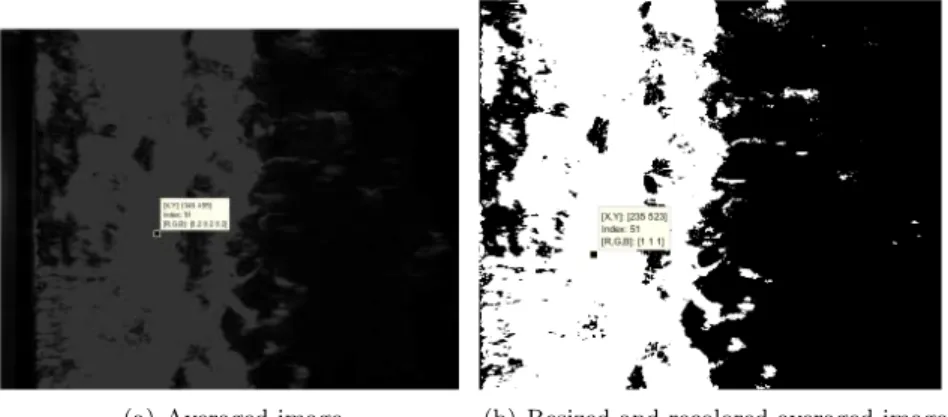
Since the size and scale of the top and side view images do not match, the image files are resized and rescaled. The parameters for these steps, the locations of the foil and cavity edges, are generated in the first MATLAB script. The first step is to resize both images. In the top view everything in front of the leading edge is eliminated. In the side view, everything below the upper edge of the foil, before the cavity inception point and a part of the image top is eliminated. Both images will only show the cavity now. For the top view, the input before resizing: figure 4.7(a) and the result after resizing, figure 4.7(b) are shown.

(a) Averaged image (b) Resized and recolored averaged image

Figure 4.7: Processing of the averaged images

The next step is to recolor the images. Processes are different here for the top and side view since different output is required. For analysis of the top view images, pixel intensity values are required. Whereas it is sufficient to know the number of white colored pixels from the side view. A conversion to binary images is performed for both images. After that:

(11)

• The white pixels in the top view are substituted by their original color values. The black pixels remain black, this is done to eliminate spurious effects of the background. The result is a black background with the cavity pixel values ”printed” on top of this background.

The input and results of this recoloring step can, be seen in figure 4.7(a) and figure 4.7(b).

Using the dimensions of the foil in pixels, and the dimensions of the foil inmm. Themm/pixel ratios for both views are obtained. The top view image is rescaled by the ratio between the top and side view image using a MATLAB ”imresize” command.

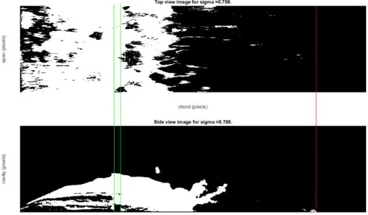
In figure 4.8 the result of the rescaling process is shown. In both images, the inception point of the cavity is at the same location. The obstacle is indicated with a green line. In the top view image, the obstacle effects become visible in the top view just after the obstacle location. This is in accordance with observations from experiments. The red line indicates the trailing edge of the foil. Based on this, it is concluded that the rescaling is performed in a correct way. Another example can be seen in figure 4.10. Since the preprocessing of the images is completely finished. The cavity height and pixel intensity can be determined from the images shown in 4.8.

Figure 4.8: Rescaled top and side view.

4.5.2. Final image analysis

Figure 4.9: Cavity height (left) and maximum pixel intensity (right)

(12)

The maximum pixel intensity is obtained from the top view by finding the maximum pixel value along the columns of the image matrices for each row (x-coordinate). The results can be seen in 4.9. Using equation 4.1, the cavity height and therewith the volume can be calculated.

4.6. Graythresh

The method of determining the cavity volume heavily depends on the graythresh use by MATLAB. The graythresh is basically a threshold which determines which pixels will become white and which pixel will become black when a color image is converted to a binary image. Since the top view images are very dark and the side view images 4.10 are very light colored, it is not possible to use the same graythresh.

The process of choosing the graythresh is done by MATLAB by the command of ”graythresh” resulting in a different threshold for the top and side view. However determined using the same method! To show the effects of the graythresh on the cavity volume, the results are shown in figure 4.10.

Figure 4.10: Original top view (left, top), top view rescaled and recolored (right, top), original side view (left, bottom) and processed side view (right, bottom)

(13)

Chapter 5 Results and discussions

5.1. Volume-time behavior, results

The volume-time output, resulting from the MATLAB analysis is classified in four ranges of cavitation numbers. The effects of the obstacles can be studied by comparing the volume-time behavior for every obstacle position. The results can be seen in figure 5.1. In every range of cavitation numbers, at least one experiment for every obstacle was available.

The volumes are largest for the lowest cavitation numbers.The volumes decrease for increasing cavitation numbers which is in agreement with cavitation theory. From figure 5.1, it can clearly be seen that every obstacle contributes to a decrease in cavity volume. The decrease in cavity volume is always lowest for the obstacle at 30%CLand highest for the obstacle at 37%CL1_{, the latter is in agreement with the results of Kawanami et. al [4].}

It is important to notice that most volume-time plots are fluctuating around a straight horizontal line. From this, it can be concluded that the cavities were stable during experiments. It has to be noticed that it is hard to maintain constant cavitation numbers during experiments. Sometimes experiments were subjected to a sudden change in cavi-tation number.

5.2. Volume-time behavior, discussion

It is remarkable to see that the obstacle at 37%CLwill always result in the highest volume reduction. On the contrary the obstacle at 30%CL will always result in the lowest cavity reduction. The other obstacles, at 26,34 and 40%CL

result in comparable values for volume reduction between the minimal (30%CL) and maximal (37%CL) values found in the experiments. The results imply that there are possibly more obstacle locations which will result in minimal and maximal cavity reduction. Therefore, it is of interest to investigate what the obstacle effects are below 26%CL and above 40%CL. Furthermore, it could be interesting to investigate whether there is a relation between the mechanism of cavity break off and the optimal obstacle location.

5.3. Cavity frequency, results

From the volume time behavior, the characteristic frequencies of the cavity volume-time behaviour can be determined. This is done by applying a fast fourier transform (FFT) to the volume-time data. The results are shown for the lowest (figure 5.2(a)) and highest (figure 5.2(b)) cavity numbers. The the frequency values belonging to a certain |V ol(ω)| peak are assumed to be the dominant frequencies in the specific experiment.

The first that can be noticed are the sharp intensity peaks for the foil without obstacle. This is in agreement with the highly periodic behavior that can be seen in figure 5.1. For the largest cavities, the peaks are positioned around 14Hz. When the cavity numbers decrease the frequencies become higher, up to 17Hzfor the last two sets of cavitation numbers. The foil with the 30%CL has approximately the same behavior although the peaks are less sharp and positioned at slightly lower frequencies. Furthermore, the behavior is more noisy what indicates a less regular cavity pattern.

When the frequency plots for the other obstacles are examined, there are still sharp peaks visible, these are however not as dominant as the peaks found for 0%CLand 30%CL. This indicates a behaviour that is far less regular. For the highest cavity numbers no peaks are visible any more.

5.4. Cavity frequency, discussion

From the results, it can be concluded that all obstacles are useful in reducing the periodic behavior of the cavities. The peak intensity is reduced for every obstacle, implying that the periodic behavior becomes less dominant. For the lower cavitation numbers, the peaks for the 26,34 and 40%CL foils have lower intensities and therefore the volume behavior is assumed to be less periodic. The 37%CL foil has two peaks very close to each other, which practically means that no clear periodic behavior can be observed any more. Furthermore, the intensity-frequency plots have more

1_{It has to be stressed that due to the camera settings, the trailing edge of the hydrofoil was not visible during the experiments with}

(14)

small fluctuations compared to the flat foil.

For the higher cavitation numbers, it looks like the periodic behavior is completely absent for the 26,34,37 and 40%CL

(15)

Figure

5.1:

Final

results

fr

om

the

me

asur

(16)

(a) Frequency output for theσ= 0.600−0.700 range.

(b) Frequency output for theσ= 0.760−0.780 range.

(17)

Chapter 6 Recommendations

As a result of the experiments, and the MATLAB code, there are a few recommendations. In my point of view, the most important improvement for the experiments would be to increase consistency. There are many variables which change from experiment to experiment which make the experiments less reliable.

• Since the camera setup has to be rebuild every new set of experiments, it is not possible to film the foil from exactly the same locations and under the same angle. Furthermore, angles and locations were changed accidentally during experiments. Both the side and top view are affected by this. To solve this problem, firm camera clamps should be used which can be calibrated in a more reliable way.

• During the experiments, some adjustments had been made to the camera aperture and light sheet distribution. Therefore the brightness of the images varied between experiments. It is highly recommended to determine a suitable light sheet and camera aperture before the experiments get started and hold to these settings during the complete set of experiments.

• It was relatively easy to determine the zoom rate of the side view camera since trailing and leading edge of the foil can easily be identified. For the top view it was more difficult since it is not possible to film the entire span of the foil due to the edges of the tunnel.Every build up of experiments, it was tried to film as much of the foil as possible. For future experiments it is recommended to make markings to the top window. In this way the same area of the top view can be filmed consistently.

• Not all slots had the same clearance with the foil, this caused some small obstacles at the foil surface. For a new foil it is recommended to insert the slots before the last stage of milling the foil in the workshop. In this way, the slots can be milled together with the foil which will result in a surface that is more smooth.

• The resulting images are disturbed by light reflections from the setup itself. In example: a screw in the rear wall of the tunnel contributes highly to the cavity volume. It would be wise to give this tunnel a thorough paint job.

• To achieve certain cavitation numbers in the tunnel, the static pressure and flow velocity were both changed. In future experiments is might be wise to change only one parameter, either the static pressure or the flow velocity. In this way the cavity volumes are not affected by the velocity of the shear flow.

6.1. There are a few remarks about the MATLAB script made by the author. Due to limited time and a lack of MATLAB experience, there are a few proposed improvements that could be done.

• In the code, some steps are not useful anymore (but were useful in the past) these steps could be eliminated to speed up the analysis.

• It would be useful to optimize the MATLAB code. When optimized MATLAB will be more efficient with time and memory. In this way it will probably be possible to analyze all of the recorded data (1 minute).

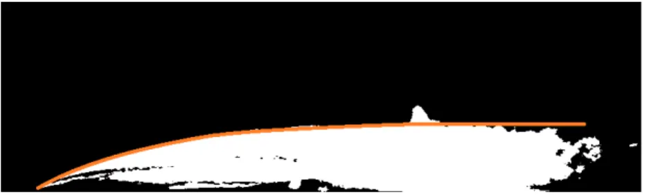
• Especially the side view images suffer from reflections and spurious bubbles. It has already been tried to identify the cavity edge from the side view and to eliminate everything that is above this cavity edge, figure 6.1. In this way only the cavity itself will be taken into account. The cavity edge can probably be described as summation of square root functions, according to the author.

• It might be interesting to determine the fraction of the entire period, required for the re-entrant jet to travel to the leading edge. In a comparison with the foil without obstacle, it can be seen whether the re-entrant jet is delayed. According to the book written by Franc and Michel [2], this fraction can be obtained with the use of the Strouhal number, equation 6.1.

St= f l

v∞

(6.1)

(18)

characteristic time required for the re-entrant jet to reach the leading edge is therewith l/v∞. The characteristic time for the entire cycle is the period which is 1/f. This Strouhal number would give a good indication of the effects of the re-entrant jet delay by the obstacle.

Figure 6.1: Example of an approximation that could be made to eliminate spurious effects, above the orange line, a reflection of an screw can be seen.

6.2. Recommendations for future experiments

• The hydrofoils used are perfect for combination of two or more obstacles, it might be interesting to see what the effects of more obstacles are. Especially in this case, it will be really of interest to measure the drag force.

• The obstacle height can be a critical factor in reducing the cavity volume. In these experiments the same obstacle height was used for every experiment. Especially for drag reduction in non-cavitating circumstances, it will be interesting to use the smallest obstacle.

(19)

Chapter 7 Other activities during the training period

During my period at the department of flow control, a few meetings were organized in which I was allowed to join. In these meetings usually all graduate students of the department joined.

7.1. Meetings

Every Wednesday evening meetings are on the program in which all graduate students of teacher Zhang (flow control), teacher Deng (Biomimics) and teacher Pan (Flow control) join. Usually the students give a presentation about the progress of their research and students and teachers will ask questions. I gave a presentation about my work for two times, and received a lot of questions and feedback. During these two meetings I stayed after my presentation and tried to understand the other presentations which were usually held in Chinese. I think that we should have these kind of meetings at the University of Twente as well, since they really contribute to the progress of the work.

7.2. Trip to Zhoushan

When I was is China for a few weeks, a trip to the city of Zhoushan was organized. Zhoushan is a city/island, three hours by bus southeast of Hangzhou. All students from the department of flow control could join in this 2-day trip, which was organized by one of the students. During the trip we visited the department of the Zhejiang University at which the Marine education and research was located. Besides this we visited the beautiful coastal areas of Zhoushan which made me realize that China has in fact lots of beautiful nature. After a perfect sea-food dinner, a few songs at the beach and a good sleep we went to peach-flower island where we saw more nature. For me, this trip was a perfect occasion to meet more people who are at the department of flow control.

Figure 7.1: Having a feet-bath in the yellow sea at Zhoushan

7.3. Teaching at the water tunnel

As part of a course in experimental techniques, undergraduate students of the school of aeronautics and astronautics visit the labs belonging to this school. Since our cavitation tunnel belongs to these laboratories, the students visited our lab in a few groups. Chen ming figure(7.2(a)) told them everything about the cavitation tunnel and we demonstrated how an experiment was performed. After this demonstration I gave a short presentation (figure 7.2(b)) about our method of analyzing the high speed images. After this presentation there was some interaction with these students about our experiments and the methods we use. Especially their knowledge of statistics is by far better compared to the knowledge of statistics of the average Dutch student. Furthermore, the good quality of their English of these students really surprised me.

7.4. Conference in Wuxi

(20)

Figure 7.2: Teachers Chen Ming (left, most right person) and Cijsouw Wout (right) giving a demonstration to undergraduate students

place in Wuxi at the CSSRC facilities. Wuxi is located a two hour train drive to the north from Hangzhou. During this meetings, employees of the CSSRC and teachers and students from both universities held presentations of about one hour. During each presentation a scientific research performed elsewhere in the world was discussed. During the presentations a lot of question were posed and there was a lot of discussion. To my personal disappointment there were only a few presentations in which the presenters discussed their own research.

For me this weekend was really interesting although I could only understand very little of what was said during the presentations. Furthermore, the food at CSSRC is really good and the hotel was really comfortable! It was really nice to be with the people from my department and I met really interesting people from the CSSRC.

(a) Presentation about the research performed by Ganesh [3] during the Wuxi conference, given by Chen Ming

(21)

Chapter 8 Appendices

8.1. MATLAB manual

8.1.1. BoundariesLocation.m

During the experiments, all images are saved in a folder belonging to the obstacle location and cavitation number of the specific experiment. The top view and side view images are saved in respectively the TV andSV folder.

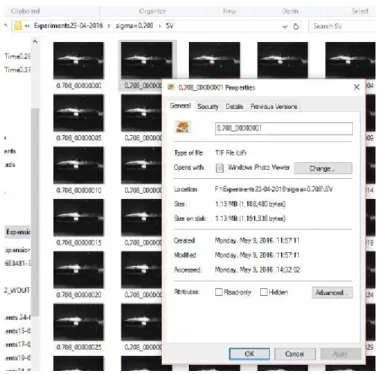
Using thePhotron andHXLink software, the images have to be converted to .tiff images. It is important to save the images using the correct filename, otherwise MATLAB will not be able to find the required images and result in an error. An example of this filename can be seen in figure 8.1. For analysis, a third folder,Results is required. When the images and results are stored in this way, MATLAB will be able to find the correct image files.

When running ”BoundariesLocation.m”, MATLAB will ask for the file location, desired number of images and the cavitation number. When these details are known, MATLAB will start calculating the average of the side view images. The filename should be of the form: ”G:\Experiments\Experiments15−04−2016\0.694” when fed into MATLAB. The programme is able to find the top view, side view and results folder by itself, as long as they exists.

Figure 8.1: Images should be stored this way for proper detection by MATLAB.

The results generated in the first script will be saved in the ”Results” folder together with some image files.

The next script, ”imagesaverage.m” requires slightly more user defined information: file location, number of files, user defined averaging number (usually chosen 5) and the cavitation number. Every averaged image is saved into a structure. These structures will be saved in a .mat file.

The last script, ”BubbleVolume.m” requires only the file location as input since other variables have been saved in the scripts before. All results will be stored in the results folder belonging to the file location.

(22)

(23)

Figure

8.3:

Dr

awing

of

the

foil

and

an

(24)

Bibliography

[1] E. J. Foeth, C. W. H. van Doorne, T. van Terwisga, and B. Wieneke. Time resolved piv and flow visualization of 3d sheet cavitation. Experiments in Fluids, 40:503–513, 2006.

[2] Jean-Pierre Franc and Jean-Marie Michel. Fundamentals of Cavitation, volume 76. Kluwer academic publishers, 2005.

[3] Harish Ganesh and Steven L. Ceccio. Bubbly Shock Propagation as a Cause of Sheet to Cloud Transition of Partial Cavitation and Stationary Cavitation Bubbles Forming on a Delta Wing Vortex. 2015.

[4] Y. Kawanami, H. Kato, H. Yamaguchi, M. Tanimura, and Y. Tagaya. Mechanism and control of cloud cavitation.

Journal of Hydrodynamics, American Society of Mechanical Engineers, 119:788 – 794, 1997.

[5] T. M. Pham, F. Larrarte, and D. H. Fruman. Investigation of unsteady sheet cavitation and cloud cavitation mechanisms, 1999.