Improved coupling Pharos Diffrac : including spatial variations in wave conditions along a ship's hull in dynamic mooring analysis

(1)

IMPROVED COUPLING PHAROS-DIFFRAC

Including spatial variations in wave conditions along a ship’s

hull in dynamic mooring analysis

(2)

2 ARCADIS NEDERLAND

DEPARTMENT OF PORTS AND HYDRAULIC ENGINEERING Supervisor: M.P. Bénit

UNIVERSITY OF TWENTE

FACULTY OF ENGINEERING TECHNOLOGY CIVIL ENGINEERING

Supervisor: C.M. Dohmen-Janssen

01-07-2016

(3)

3

Preface

This thesis report is the final result of the graduation project to complete my bachelor degree in civil engineering at the University of Twente. The report presents a research which has been performed at the ports and hydraulic engineering group of Arcadis Nederland. My supervisor has given me the opportunity to work on a project on which the whole group was involved. The research involves a study to different ways of calculating the mooring conditions of a ship. The whole process of calculating mooring

conditions involves a large amount of theories and different numerical models. Due to this, a lot of help was needed to find a way to complete the research. This has brought me a great amount of new

knowledge. Besides this, I have improved a lot of soft skills. I would like to thank my supervisors: Matthijs Bénit (Arcadis) and Marjolein Dohmen-Janssen (University of Twente) for the feedback and giving me direction in the research. I also would like to thank the colleagues from the ports and hydraulic engineering group for all their help, support and feedback. Special thanks to Jurjen Wilms for sharing his knowledge and making time for answering all my questions.

(4)

4

Abstract

A moored ship is subjected to different forces. When the conditions are too extreme, the lines can break and dangerous situations will occur. The time ships are not able to operate is defined as the down-time. During the down time of a ship, no cargo can be (un)loaded, therefore this time is expensive for port operators and

shipping lines. In operational perspective, harbors are interested in the downtimes of their ships and in methods to reduce the down-times of ships in their harbors. On the other hand in design perspective, in the processes of designing ports these down-times are important to consider.

To calculate mooring conditions, it is required to consider all relevant forces that act on a ship. Two forces have a dominant influence on the ship. Firstly, forces caused by waves (wave forces). These forces are applied to the ship’s hull. The second type of forces acting on the hull of the ship are the fluid reaction forces. These forces are caused by the motions of the ship itself. These types of forces can be split up into two parts: the added mass and the damping. The added mass is caused by the water around the ship being set in motion which will cause some extra moment of inertia. The damping forces are caused by the damping motions of the ship (Vis & Benit, 2016).

For calculating mooring conditions (motions and line forces) three models have been used: A wave penetration model (PHAROS), a 3D ship diffraction model (DIFFRAC) and a dynamic mooring model (MOORINGS). A simplified but common methodology exists to calculate mooring conditions by using all three of the models, however this method brings uncertainties in output because the spatial variation of wave conditions along the hull of the ship is not taken into account. It is expected that the spatial variations of wave conditions along the hull of the ship have a significant impact on the mooring conditions. In certain conditions, the existing method only considers the wave conditions at one location on the hull of the ship. A method has been developed to consider the spatial variations of wave conditions along the hull of the ship. This has been done by coupling the wave potential model (PHAROS) to the hydrodynamic ship diffraction model (DIFFRAC) in a direct way.

The aim of the research is to contribute to the development of a more realistic representation of mooring conditions in a dynamic mooring analysis. This is done by answering the question of: what is the most accurate way of connecting the models PHAROS and DIFFRAC for calculating the mooring conditions? This main question has been answered by performing a dynamic mooring analysis for the existing method and the newly developed coupling method. For determining the most accurate method, a third reference method has been included. This method calculates the mooring conditions in the most ideal way. This is achievable by excluding bottom depth variations in the analyzed situations.

To get an indication of the working of the coupling, the wave forces have been calculated in DIFFRAC for the coupling method and the reference method. From a comparison, it became clear that the coupling method followed the trend of the ideal situation, however for higher frequencies the relative error became larger. The coupling method and the existing method have been compared with the MOORINGS output. From this output it became clear that the newly developed coupling method is the most accurate method for calculating the mooring conditions. However the effect of the improvement using the coupling is not significant. This can be clarified by the fact that calculations are based on wave conditions with a wave height of one meter. For more extreme situations it is expected that the results from the coupling method show significant improvements in comparison with the common method. It can be concluded that the new developed coupling theory has big potential to become the standard way of calculating mooring conditions in a dynamic mooring analysis. The current research is based on a situation with ideal conditions, and many simplifications have been made in this research. This decision has been made to get a pure comparison between the methods. However, for future research it is recommended to investigate whether the coupling will also generate the same

(5)

5

1.

Introduction

In this section an introduction of the research is given. First of all the context of the problem is described. In section 1.2 the research aim and question is stated. In section 1.3 the used methodologies are described. This chapter ends with a description of the outline of the report, which can be used as a reading manual.

1.1. Problem context

During storm conditions, waves have a dominant influence on the movement of a ship. In the case of moored ships, it is important that these vessels can be tied down to ensure they will have a safe stay in the harbor. In the case of designing harbor structures, it is required to assess the wave conditions that can penetrate into a port area under design storm conditions which will have an influence on the movement of the ship, and the lines which form the connection with mooring structures. These lines do not have infinite strength, under certain conditions it is impossible to guarantee that the lines can withstand the forces caused by extreme wave conditions. The time in which ships cannot moor is defined as the down-time. During the down time no cargo can be (un)loaded, therefore this time is expensive. In operational perspective, harbors are interested in the down-time of their own ships and in methods to reduce the down-time. On the other hand in design perspective, in the processes of designing ports the down-times of ships are important to consider.

To calculate mooring conditions, it is required to consider the different forces that act on a ship. In the case of mooring, two forces do have a big influence on the ship. Firstly, forces caused by waves do have an influence on the motions of the ship. These wave forces act on the ship’s hull. The second type of force acting on the hull of the ship are the fluid reaction forces, these forces are caused by the motion of the ship itself. These types of forces can be expressed as two components: The added mass and the damping. The added mass is considered because the water around the ship will cause some extra moment of inertia. The damping forces are caused by the damping motions of the ship (Vis & Benit, 2016).

In this research the mooring conditions are defined as the motions of the ship and the forces on the mooring elements caused by the ship. In this study the focus is applied on the on the motions of the ship. The motions of the ship are visualized in Figure 4. The process of calculating the mooring conditions (the motions of the ship), can be described as a dynamic mooring analysis (DMA). The DMA performed in this research consists of a combination of three models. A short description of the models is shown below (for a more complete description of the models, see section 2).

1. Wave penetration model (PHAROS): Evaluating the wave conditions at the moored ship location. 2. 3D hydrodynamic ship diffraction model (DIFFRAC): Evaluating the wave forces on the

unrestrained ship from monochromatic wave conditions with various frequencies and directions. The wave conditions are translated to forces, displacements and rotations of the ship.

3. Dynamic mooring model (MOORINGS): Evaluating the motions and forces of the moored ship to the mooring conditions using a dynamic mooring model (DMA). In this model the

(8)

8

1.1.1. Previous way of calculating mooring conditions

A method is available for using the three models (described above) for performing a DMA. This method converts wave conditions to mooring conditions in the harbor. The inaccuracies of this method have been studied in this research by performing a study of a ship in sheltered area. It is expected that this way of calculating mooring conditions causes considerable errors because the wave climate is not well represented.

1.1.2. Improved methodology of calculating mooring conditions

With a more realistic representation of the wave climate, a better estimation of the down-times can be made. Also in design processes of new harbors, effects on ship motions can be predicted and a better harbor layout design can be made. There are different ways of applying and connecting these models to each other to calculate the mooring conditions. A new method have been developed in which the inaccuracies have been reduced. For the newly developed method of connecting the three models it is expected that the spatial variation of wave conditions around the hull of the ship can be taken into

account. In the existing method, the wave conditions are grasped at the center of gravity of the ship. From this, the ship motions are calculated. It turned out that wave conditions vary along the hull of the ship. By calculating the forces along the hull (spatial variation), a more realistic mooring condition can be

calculated.

The whole research consists of a detailed analysis of the existing method, the newly developed method and a reference method to calculate the mooring conditions. This research is about the effect of the new invented calculation method, and how it can be optimized.

1.1.3. Interests for Arcadis

(9)

9

1.2. Research aim and questions

The main objective of the research is to contribute to the development of a more accurate representation of mooring conditions in a dynamic mooring analysis. The development consists of including the spatial variation of wave conditions along the ship hull instead of prescribing uniform conditions (e.g. those at one specific point). This is done by coupling the wave penetration model (PHAROS) to a hydrodynamic ship diffraction model (DIFFRAC). The objective of this research is to identify the most accurate way to connect the models, and determine the effect of the new strategy of calculating mooring conditions by applying the coupling between the models PHAROS and DIFFRAC. This is done by making an assessment of different calculation methods to calculate the mooring conditions. The main research question is:

What is the most accurate way of connecting the models PHAROS and DIFFRAC for calculating the mooring conditions? (1)

Before answering the main question, first some information about the different models and the coupling theory needs to be collected. In the research there will be a focus on the theory behind the different models, and the different elements which connect the models to each other. The question is:

What are the different elements used in the coupling and the connection of the models, and what is the consistency between the different elements? (1.1)

The main objective of the research is to develop a more accurate representation of mooring conditions in a dynamic mooring analysis. For this aim it is important to consider the differences between the

developed coupling method and existing method in which PHAROS and DIFFRAC are used to study the mooring conditions. First of all the results of these different calculation methods will be analyzed. The sub question is:

Which calculation method is the most accurate to represent the mooring conditions? (1.2)

After analyzing the different methods, a special focus will be applied on the method in which the newly invented coupling is involved. In this sub question the effect of the expected improvement will be determined. There will be also tried to justify the distinction in results between the coupling method and the other calculation methods. The sub question is:

What is the effect of the newly invented coupling method in comparison with other calculation methods? (1.3)

During the whole research, special attention is paid to the improvement and automation of the modelling process. It is important to mention that the research is not only based on the coupling. This research is also based on studying ways how the coupling can be improved. Will it be possible to apply the coupling in other cases? The last sub question is:

(10)

10

1.3. Methodology

In this chapter an overview of the used methods is given. Applying these methods will provide an answer to the different research questions.

1.3.1. Literature methods

Basic theoretical knowledge about waves is important to have before starting the research. In this research, wave behavior in harbors will be modelled, researched and analyzed. To interpret the output of the model and the working of the model itself and get understanding of linear wave theory different literature sources have been studied. The literature and background principles of this research are mainly based on two literature sources:

Table 1: Main literature sources

Title Author Volume Year

Waves in oceanic and coastal waters

L. H. Holthuijsen 387 2007

Wind generated ocean waves I. R. Young 288 1999

1.3.2. Calculation methods

Three different calculation methods have been studied in this research. Each method combines the required modelling steps in a certain way to calculate the mooring conditions in the mooring model (MOORINGS). Method number two involves the newly developed coupling. After performing an assessment of the different methods, the main research question can be answered. For a good assessment of the coupling and different calculation strategies, one layout is considered for the different methods. The situation involves a ship behind a detached breakwater. In the cases the breakwater is used in the models, the ship is placed at three different positions behind the detached breakwater (The positions are named as L1, L2 and L3 and defined in subsection 1.5.3). These positions have been chosen in such way that the wave conditions at the different points at the hull show a big difference. This in order to

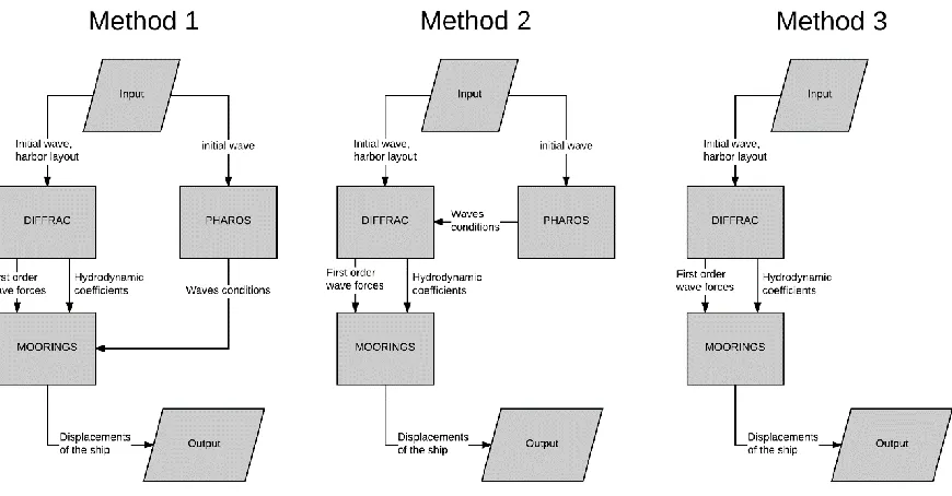
determine the effect of taking into account spatial variations along the ship’s hull. The different calculation methods are visually presented in Figure 1.

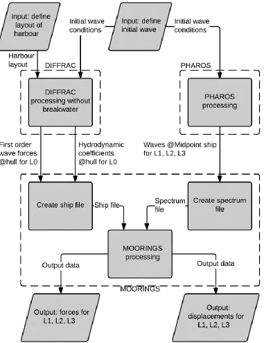
Method 1

In the first case the wave conditions at the center of gravity of the ship is obtained from the PHAROS model. In DIFFRAC the ship’s behavior is modelled without a breakwater (ship in open water), but the wave forces and fluid reaction forces (also stated as the hydrodynamic coefficients) is calculated at the hull around the ship. The mooring model (MOORINGS) is used to apply the wave condition (from PHAROS), using the corresponding wave force and fluid reaction forces (from DIFFRAC). With these inputs, MOORINGS is used to calculate the mooring conditions. This method is the common method of calculating mooring conditions at Arcadis. This method has been chosen to asses if there are differences in results with the coupling method.

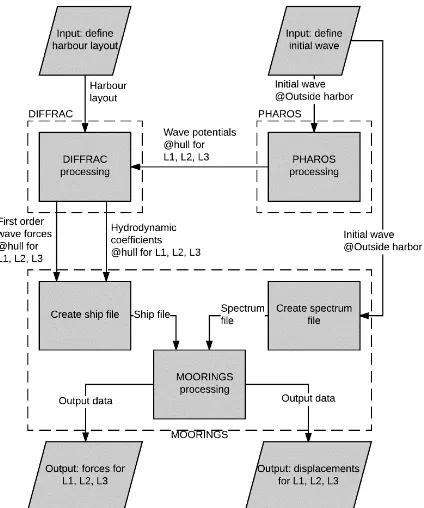
Method 2

(11)

11 conditions along the hull of the ship into forces which act on the ship’s body. In this way the wave forces is calculated. MOORINGS is used to evaluate the resulting mooring conditions.

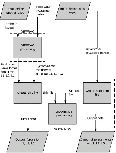
Method 3

[image:11.612.89.524.277.504.2]

Method 3 has been included to consider because this method does not use PHAROS for the wave conditions. In this research a specific situation is considered with uniform depth (ship behind detached breakwater). For this specific situation it is possible to do the calculations only with DIFFRAC and MOORINGS. In general DIFFRAC is able to generate the wave conditions as a standalone model. It will be interesting to see if this exclusion of PHAROS will cause differences in results. DIFFRAC is used as an input for MOORINGS for the wave conditions, wave forces and hydrodynamic coefficients. This method has been added because it describes the ideal situation for this case. This calculation method has been added as a reference. Note that for other cases this referential method would not be able to generate results with the specification of an ideal situation. Therefore only in the situation used in this research, method 3 can be used as a referential method.

(12)

12

1.3.3. Methods for analysis

Below the process of analysing the obtained results is described. The analysis of the working of the coupling method consists of several steps. As described in subsection 1.3.2 it has been described that several models have to be run for getting an complete assessment of the different calculation methods. The analysis process is based on checking the validity after each step. When it turns out that after a modelling step the output is not right, it is not valuable to continue with the research process. For this reason many validation checks have been performed in this research process. Below, the process is described of the different analysis steps which have been performed in this research.

The first goal is to get an indication of the working of the coupling. To make a first comparison analysis the results can be compared based on the wave forces coming from DIFFRAC. After this first indication of the working of the coupling, the remaining computation have to be performed. The steps for finishing the analysis of the research are shown in Table 2. For the detailed visualization of the whole modelling process see section 2.4.

Table 2: Analysis steps performed in the research

Step Nr.

Activity Type of

activity

Reference chapter

1. Run PHAROS for method 2 and 3 Modelling Section 2.1 and 3.1 2. Validate the PHAROS results for method

2 and 3

Analysis Subsection 4.1.1 3. Run DIFFRAC only for method 3 Modelling Section 2.2 and 3.2 4. Validate the DIFFRAC results for method

3

Analysis Subsection 4.2.1 5. Couple potentials from PHAROS and

apply in DIFFRAC

Modelling Section 3.3

6. Run DIFFRAC for method 2 Modelling Section 2.2 and 3.2 7. Compare DIFFRAC results for method 2

and 3.

Analysis Subsection 4.2.3 8. Run PHAROS for remaining cases Modelling Section 2.1 and 3.1 9. Validate the PHAROS results for

remaining cases

Analysis Subsection 4.1.1 10. Run MOORINGS for the three different

methods

Modelling Section 2.3 and 3.4 11. Compare MOORINGS results for method

1, 2 and 3

Analysis Section 0 12. Formulate conclusion about the coupling

based on MOORINGS results

(13)

13

1.4. Outline of report

Section 2 is dedicated to the process of a dynamic mooring analysis. In this section the different involved models are described in further detail. Included is a description of the theoretical principles on which the models are build. The answer of research question 1.1 is mainly based on this chapter.

(14)

14

1.5. Definitions and conventions

1.5.1. Units

All parameters and variables have units according to the international SI conventions. The unit for wave frequency is in rad/s. The conversion of this unit to Hz, and the calculation of the wave period is shown below.

𝑓 = 𝜔 2𝜋 𝑇 =2𝜋 𝜔

With:

𝑓 Wave frequency in Hz.

𝜔 Wave frequency in rad/s.

𝑇 Wave period in s.

1.5.2. Wave directions

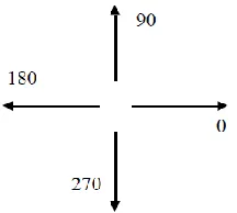
[image:14.612.96.204.344.441.2]

The wave directions are defined with the polar coordinate system. This means that a wave coming from the south corresponds with wave direction of 90 degrees. This is visualized in Figure 2.

(15)

15

1.5.3. Ship positions

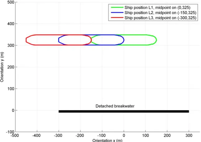
Three different ship positions will be considered. The origin of the orientation has been positioned in the midpoint of the ship on position L1. The ship is orientated with the bow in direction of the positive side in each case. The different ship positions are visualized in Figure 3.

Figure 3: Positions of the ship related to the breakwater

1.5.4. Ship motions

[image:15.612.73.397.139.368.2]

The ship motions used in this research are defined in Figure 4. Most important motions for this research are surge, sway and yaw.

Figure 4: Definition of ship motions (Arcadis, 2015)

1.5.5. Notations

The following notations are used in this report:  Decimal point. Thus 1.5 means one and half.

 Digit grouping symbol. Thus 12,000,000 means 12 million.

(16)

16

2.

Dynamic mooring analysis

A dynamic mooring analysis is one of the processes of calculating mooring conditions of the ship. For this process different methods and models can be used. In this section, a description is given of the involved models in this research to perform a dynamic mooring analysis. This section will end with a visualization of the data flows between the models. In this way the collaboration of the models and the data flows will be understood.

2.1. PHAROS model theory

The PHAROS model has the function to evaluate the wave conditions in the harbor. This wave

penetration model (WPM) simulates the waves which propagate from the sea into the harbor. In general PHAROS investigates the effectiveness of the harbor design before construction (Reijmerink, n.d.). One of the features of the PHAROS models the fact that this model is able to consider the bottom depth variation. In this research this will not be considered. This in order to create an optimal comparison between the different calculation methods.

2.1.1. Calculating wave potentials

To describe wave processes used in PHAROS (and DIFFRAC), four components need to be determined. The three wave velocity components (speed in 3 directions: u, v and w) and the pressure on a specific point. To find these values four equations have to be solved (Continuity equations, Navier Stokes

equations, Laplace equations and the Bernoulli equation). The derivation of these equations can be found in appendix A.ii.

The four parameters described above can be expressed in one function, the velocity potential function. The analytical expressions for particle velocities (u, v and w) and the wave-induced pressure in the water are found with a mathematical technique that uses a rather abstract mathematical concept (Holthuijsen, Waves in oceanic and coastal waters, 2007). In other words, this potential function (or the value for potentials) describes the three velocity components and the pressure in the water. The values for potentials are the main output of the PHAROS model.

2.1.2. Grid and wave penetration

Before modelling waves in PHAROS a grid has to be defined. With the finite elements method the wave conditions all over the grid points are calculated. For these penetration of waves all over the area,

reflection and diffraction principles are considered. The principles of these processes have been described below.

(17)

17 on the phase of the wave at the position of the wall, it can occur that the resultant wave will be fully disappeared, this has been visualized in Figure 6.

Figure 6: reflection on a wall (phase difference: 0.5*pi)

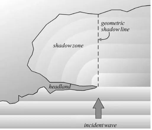
[image:17.612.73.330.406.625.2]

Wave diffraction will occur when a wave moves beside an object. Because of this object the wave will diffract and change direction. Diffraction causes changes in the amplifications and directions of the waves. In the case which is visualized in Figure 7 an incident wave is coming from the south. Because of the headland a shadow zone will occur. If the diffraction process would be ignored, the waves would reflect against the headland and no waves would be observable in the shadow zone. However, with diffraction accounted for, the waves curve into the shadowed area behind the headland as can be seen from Figure 7 (Holthuijsen, Waves in oceanic and coastal waters, 2007).

Figure 7: visualization of diffraction process (Holthuijsen, Waves in oceanic and coastal waters, 2007)

(18)

18

2.2. DIFFRAC model theory

The DIFFRAC model is used as the hydrodynamic ship diffraction model. In general this model

calculates the different types of forces on the ship. In subsection 2.2.2 and 2.2.3 this have been described. In the case of the coupling method, the input of the hydrodynamic ship diffraction model are the wave potentials from PHAROS (function which describes the four calculated components: speed in u, v, and w and the pressure). An explanation of the wave potential is given in subsection 2.1.1. These wave

potentials are converted into wave velocities and pressures which can be applied on the ship’s hull. For calculating the forces DIFFRAC makes use of a panel method. This panel method divides the ship’s hull into different panels, this has been visualized in appendix B. On each panel the potential has been calculated. With the wave potential the pressure can be calculated by applying Bernoulli’s law. By an integration of the pressure over the surface area of the panel, a force can be calculated. Summing the contributions from all panels gives the resultant wave forces on the ship at the center of gravity.

DIFFRAC is a model in which it is not common to consider bottom depth variations. As described before DIFFRAC consists of certain objects which interacts with waves. The bottom depth can be taken into account as an extra object above the ground surface in the model. This requires a lot of panels. Because of this reason it is hard to perform a run which considers bottom depth variation. In this research, the surface is considered as one flat surface. This is the big difference between the models PHAROS and DIFFRAC. PHAROS is able to consider the bottom depth variation.

2.2.1. Linear systems theory

The linear systems theory states the fact that the relationship between two variables can be treated as a linear function. In the case of waves, for example a surface elevation spectrum can be transferred to the spectrum of some other wave variable. The definition of a linear system is given in the following equation:

𝑎 ∗ 𝑥(𝑡) + 𝑏 ∗ 𝑦(𝑡) → 𝑎 ∗ 𝑋(𝑡) + 𝑏 ∗ 𝑌(𝑡) (Holthuijsen, Waves in oceanic and coastal waters, 2007)

In this equation x and y are called the excitation functions, and X and Y are called the response functions. Consider for the excitation function for example the surface elevation due to waves (x), and for X the water pressure at some point in the water. If the surface elevation will become two times bigger, then the water pressure will be doubled as well. Another characteristic of a linear system is, if the excitation function is harmonic, the response function is harmonic as well with the same frequency (Holthuijsen, Waves in oceanic and coastal waters, 2007).

2.2.2. Fluid reaction forces (added mass and damping)

The fluid reaction forces (the hydrodynamic coefficients) are defined as the forces caused by the motions of the ship itself. The water tries to resist the force of the ship. On the ship a reaction force is felt due to the resistance of the water, this is called a fluid reaction force. This theory is based on the linear behavior of systems, described in subsection 2.2.1. In this case it means that a wave with a certain frequency is coming in, and the fluid reaction force has the same frequency.

(19)

19 move some volume of surrounding fluid (Techet, 2005). The second term represents the damping. This is the resistance of the water caused by the movements of the ship itself. When a ship moves, a force will act on the hull of the ship proportional to the velocity of the ship.

2.2.3. Wave forces

(20)

20

2.3. MOORINGS model theory

In MOORINGS the different calculated parameters are coupled together. This software makes a

simulation of a moored ship. The frequency domain is transferred to motions and forces in a time domain. The main aim of this model is to contribute to the design of ship-related infrastructure. In the program environmental conditions and the mooring system is modelled as forces that act on the ship. These environmental conditions vary in time. The input of this simulation model is composed of a large number of parameters that describe the characteristics of the ship to be used, the mooring system and the

(21)

21

2.4. The interaction of the models

[image:21.612.83.464.162.656.2]

This chapter ends with a description of the working and interaction between the models. In the above described section the different models have been described. In this section the interaction of the different models have been visualized in different flowcharts, each presenting a calculation method.

(22)

[image:22.612.80.504.77.585.2]

22

(23)

[image:23.612.82.460.87.585.2]

23

(24)

24

3.

Model schematization

In this section a description is given of the set-up of the different models. For the interpretation of the results it is important that it is clear which calculations have been performed and which assumptions have been made in the modelling set-up. In this section a focus is on the fact which simplifications have been made in the models and how the models represent the real world.

3.1. PHAROS set-up

3.1.1. Determination of layout

The modelled situation will consist of a detached breakwater. A ship was placed at three different positions behind the detached breakwater. The exact positions are presented in subsection 1.5.3. The angles of incoming waves will consists of waves from directions 45, 90 and 135 degrees (polar coordinate system, see subsection 1.5.2). A visual representation of the determination of the area size is visualized in Figure 11. It have been chosen to create a symmetric layout to create a realistic situation. The bottom is considered as a flat surface, with a water depth of 21.7 m. This layout is an idealization of reality. In reality no boundaries are defined, for the PHAROS model this is required. To create a realistic situation the size of the layout has been chosen such that no disruptions will occur on the position of the ship and the breakwater. Note that no ship is modelled in PHAROS, only the ship positions are important to consider.

Figure 11: Layout in PHAROS

3.1.2. PHAROS grid

Waves with different frequencies are modelled. The type of wave which is considered is a monochromatic wave. In this case the wave frequency will vary from 0.05 till 1.6 rad/s. The omega (wave frequency in rad/s) values will increase with a value of 0.05. So 1.6/0.05=32 runs are made in each three different directions (45, 90 and 135 degrees, see 1.5.2). The grid size is determined for the lowest value of the wave period (highest frequency). A high frequency wave will need more grid points than a low frequency wave to describe a proper wave field. For the determination of the amount of grid points in PHAROS, the following points have to be determined.

Creating the grid

(25)

25 set to 7 points in a wave length. The period which corresponds to a wave with frequency 1.60 rad/s is 3.9 s (formulas used from subsection 1.5.1). The wave length is calculated by using the dispersion

relationship. The dispersion relationship gives the relation between the wave number, frequency and depth based on the linear wave theory. For a harmonic deep water wave the dispersion relationship formula can be simplified to:

𝐿 =𝑔𝑇_2𝜋2 (Holthuijsen, Waves in oceanic and coastal waters, 2007)

𝐿 = 1.56 ∗ 𝑇2_{= 1.56 ∗ 3.9}2 _{= 23.7 𝑚}_{(Holthuijsen, Waves in oceanic and coastal waters, 2007)}

Pharos makes an automatic placement of grid points based on the period of the wave. First a grid was created based on the highest frequency (period=3.9 seconds). After creating a grid it is important to consider the grid shape and size. The areas shouldn’t be far from begin equilateral. In other words, the angles of a triangle should all three have approximately the same value. The grid statistics of the created grid are presented in Table 3.

Table 3: PHAROS grid statistics

Grid statistic Value

Number of elements (-) 2,145,374 Number of node points (-) 1,075,018 Minimum element area (m) 0.0451912 Maximum element area (m) 2.48677 Frequency range (rad/s) 0.05 – 1.60

Total area (m2₎ _1.554E+6

Total volume (m3₎ _3.3721E+7

3.1.3. Boundary conditions

(26)

26

3.2. DIFFRAC set-up

In the DIFFRAC calculations four scenarios need to be calculated. As described in the methods, in the first calculation method a ship without a breakwater is modelled in DIFFRAC (L0), see Figure 8. For this, one calculation is needed (for all wave direction and frequencies). For the second calculation method (situation with breakwater) the three positions of the ship need to be modelled. In this section the set-up of the DIFFRAC model is discussed.

3.2.1. The ship’s properties

The type of ship with which the modelling in DIFFRAC and MOORINGS is performed is a Very Large Crude Carrier tanker (VLCC). A visualization of the model of the ship with the different ship views can be found in appendix B. This type of ship has been chosen because of considerable reasons:

 The shape of the is representative for a wide range of tankers.  Previous research cases have been studied with this kind of ship.

 Waves do have a big influence on these kind of ships, in comparison with other factors. The ship has a big draught, and the block coefficient is higher in comparison with other ships. The block coefficient represent the ratio between the volume of the ship itself and the volume of an imaginary body in the shape of a block which is drawn around the outer points of the hull of the ship. For a ship with a rectangular shape, the block coefficient would be one.

3.2.2. Estimation of the size of the panels of the ship

For DIFFRAC calculations, the different objects (ship and breakwater) are modelled with panels. On these panels the different pressures and forces are calculated. This idealization has been used to shorten the run time. To create a realistic and fast run, it is important to minimize the amount of panels and to create a realistic run. This is done by determining the proper panel size. This size is based on the highest wave frequency. The highest wave frequency is: 𝜔 = 1.6 𝑟𝑎𝑑/𝑠. This corresponds to a wave period of 3.9 s (subsection 1.5.1). For the calculation of the wave length, the dispersion relationship described in 3.1.2 have been used.

𝐿 = 1.56 ∗ 𝑇2_{= 1.56 ∗ 3.9}2 _{= 23.73 𝑚}_{(Holthuijsen, Waves in oceanic and coastal waters, 2007)}

As described in subsection 3.1.2, it turned out that the number of points to describe a wave properly can be set to 7 points in one wave length. The estimated panel size is calculated by dividing the wave length to seven:

𝑃𝑎𝑛𝑒𝑙 𝑠𝑖𝑧𝑒 = 𝑊𝑎𝑣𝑒 𝑙𝑒𝑛𝑔𝑡ℎ

𝑝𝑜𝑖𝑛𝑡𝑠 𝑝𝑒𝑟 𝑤𝑎𝑣𝑒 𝑙𝑒𝑛𝑔𝑡ℎ= 23.73

7 = 3.39 𝑚

(27)

27

3.3. Coupling set-up

(28)

28

3.4. MOORINGS set-up

The MOORINGS model is based on several types of input. These inputs involves the layout properties, ship properties and environmental conditions. The different inputs are brought together in MOORINGS which calculates the displacements and the forces on the lines and fenders caused by the ship. The flow of input data has been visualized in section 2.4. The different properties and conditions are described below.

3.4.1. Layout properties

The layout has been defined as the visualization of the area around the ship. This includes the harbour and the mooring structure. In the layout, the location of the different mooring elements is determined.

Basically, the layout file consists of two different parts. First the parts which are not affected by the calculation, in this case these are the jetty and the breakwater. When the calculation is done without these layout elements, the same results will be obtained. The second part of the layout is the mooring structure. These are the mooring elements such as the lines, fenders and springs. The mooring structure has been defined on the side of the shore (north side, waves coming from the south). The structure itself (position of the lines, fenders etc.) has been taken from an existing Arcadis project in Puerto Nuevo, Colombia in which the same ship was modelled.

Figure 12: MOORINGS layout for position L2

3.4.2. Ship properties

For each modelled situation the ship will respond in a different way. In MOORINGS this response of a ship in a certain situation is obtained from DIFFRAC. For validating the response of the ship, some tests have been performed. All tests are based on a free floating body. For all tests the ship’s response are calculated for all motions.

Test 1: start out of balance: Heave decay, roll decay and pitch decay (see subsection 1.5.4). Test 2: do nothing, and look what happens

Test 3: apply wind: wind from abeam and wind from head on Test 4: apply current: current from abeam and current from head on Test 5: apply waves regular and irregular waves

3.4.3. Environmental conditions

In the case of mooring a ship. Many environmental conditions can be considered (e.g. wind, wave, current conditions). In this research, only the wave conditions are taken into account. To apply the wave

(29)

29  Wave height

 Wave direction (only for method 1, see section 2.4)  Wave frequency: 0.40, 0.80 and 1.20 rad/s.

 Water depth

 Number of wave systems

 Type of waves (regular/irregular waves) Spectrum for method 1

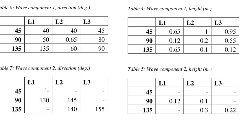
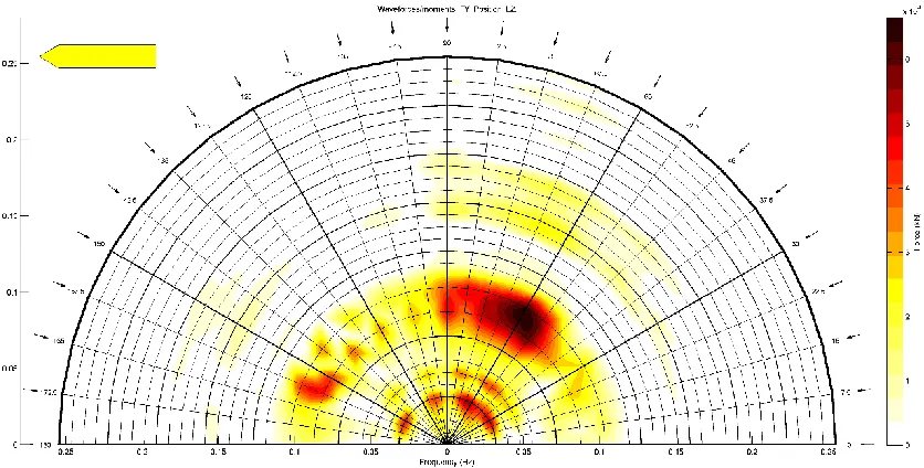
[image:29.612.78.510.342.556.2]

In method 1 the wave spectrum is based on the wave conditions at the midpoint of the ship. These data can be obtained from PHAROS. The so-called r-DPRA tool has been used to obtain the information about the wave directions and wave height at the midpoint of the ship. Because reflection/diffraction processes occur, it is necessary to represent the wave conditions with different wave directions to the midpoint of the ship in MOORINGS with a different wave height for some cases. The data which is applied in the spectrum definition for method 1 is obtained from the figures which corresponds to a wave frequency of 0.80 rad/s. Further analysis is based on the wave direction and wave height with a frequency of 0.80 rad/s. A brief overview of the values determined from the figures is shown in Table 4, Table 5, Table 6 and Table 7.

Table 6: Wave component 1, direction (deg.)

L1 L2 L3

45 40 40 45

90 50 0.65 80

135 135 60 90

Table 7: Wave component 2, direction (deg.)

L1 L2 L3

45 1- - -

90 130 145 -

135 - 140 155

Spectrum for methods 2 and 3

For method 2 and 3, the spectrum parameters in MOORINGS are obtained from the wave outside the harbor. This wave has a wave height of 1 meter. For this 1 meter wave the frequencies 0.40, 0.80 and 1.20 rad/s is performed.

1_{- means there is no second wave component taken into account}

Table 4: Wave component 1, height (m.)

L1 L2 L3

45 0.65 1 0.95

90 0.12 0.2 0.55

135 0.65 0.1 0.12

Table 5: Wave component 2, height (m.)

L1 L2 L3

45 - - -

90 0.12 0.1 -

(30)

30

4.

Results and analysis

In this chapter the results are presented. Besides this, different analyses are performed to put the results in its perspective. This chapter starts with a description of the PHAROS results. After this, the DIFFRAC results are presented. The chapter ends with a description of the MOORINGS results.

4.1. PHAROS results

The results from the PHAROS model are presented in terms of the wave height and the wave image. The wave amplification represents the ratio of the incoming wave (initial wave) and the wave height at certain locations in the layout. The wave amplification can be interpreted as the wave height for an incoming wave, with an initial value of 1 meter at certain locations in the layout. The wave image can be interpreted as a top view picture of the waves. The visual results of the Pharos runs are shown in appendix D for the lowest, mean and highest frequencies in the range.

4.1.1. Validation PHAROS results

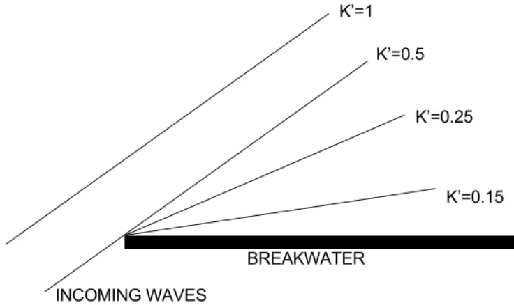
[image:30.612.81.449.448.667.2]

The validation of the PHAROS results is mainly based on the case with an incoming wave from direction 45 degrees with a frequency of 0.40 rad/s. For the validation of the PHAROS results of this specific case, different visualization checks have been performed. From the “Shore protection manual” (US army corps of engineers, 1984), different wave diffraction diagrams have been used to analyze the diffraction patterns from PHAROS. These diagrams have been conducted for a semi-infinite breakwater for different angles for incoming waves. In the case of an incoming wave with direction 45 degrees, the diffraction along these directions should have been a diffraction coefficient (K’) with a value of approximately 0.5. The diffraction coefficient can also be defined as the wave amplification. This principle has been visualized in Figure 13. From Figure 14 it can be concluded that the wave amplification output from PHAROS is in line with the principles from the shore protection manual (US army corps of engineers, 1984).

(31)

31 PHAROS is a model which is based on boundaries. The incoming boundary will generate the waves. For wave directions 45 and 135 degrees, an area will arise in the figures which is not affected by the incoming waves. For example, in the top left corner of the wave amplification Figure 14 this is visualized. For this research it is important that the ship will not be situated in this area. As can be seen in the results from PHAROS, the ship’s positions will not be in the areas which are not affected by the incoming waves.

Figure 14: wave amplification, frequency: 0.40 rad/s, direction: 45 deg

(32)

32

4.2. DIFFRAC results

The analysis of the DIFFRAC results starts with a comparison of wave amplification diagrams between DIFFRAC and PHAROS. It is required that these outputs from the models produce the same output. The main DIFFRAC results are represented as the added mass and damping and the wave forces. First of all, the added mas and damping are compared for the different ship position (L0, L1, L2 and L3). After this the analysis continues with a comparison of the wave forces. The main analysis is based on the wave forces because this is the essential point which is calculated in different ways for the different calculation methods.

4.2.1. Comparison DIFFRAC-PHAROS results

In DIFFRAC the wave amplification has been calculated. With the results of the wave amplification the comparison between the PHAROS and the DIFFRAC output can be made. When the amplification figures from PHAROS and DIFFRAC is compared, it can be seen that the ship itself in the DIFFRAC output do have a big influence on the waves. The ship in DIFFRAC behaves to some extent as a

breakwater. From Figure 15 it can be observed that the wave amplification behind the ship is remarkably lower than at the front. Also the reflection of the ship causes a chaotic wave pattern between the

breakwater and the ship, this is the result of the wave reflection of the ship.

In contrast with PHAROS, in DIFFRAC outer boundaries will not be defined. This means that over the whole area waves can be observed as can be seen in Figure 15. This is in contrast with the PHAROS results. The wave amplification figure from DIFFRAC (case without ship) has been directly compared with the PHAROS results in Figure 16. In the upper left corner big changes in wave amplifications are observable between the models. This is due to the fact that PHAROS defines boundaries and in this area now waves occur produced by the wave exciter boundary. A second notable observation which can be made from Figure 16 is the chaotic pattern on the right side of the breakwater. This pattern is presumably the consequence of a misstep in defining the breakwater layout in the PHAROS set-up. However, as can be seen from Figure 16 the effect of this misstep is small on the waves which occur on the positions of the ship. The figures which involves the comparison of DIFFRAC and PHAROS for the specific case of 0.40 rad/s can be found in appendix E.ii.

(33)

33

Figure 16: Difference in wave amplification DIFFRAC - PHAROS, frequency: 1.60 rad/s, direction: 45 deg.

4.2.2. Added mass and damping

The second results which are obtained from DIFFRAC are the hydrodynamic coefficients. The hydrodynamic coefficients are divided in the added mass and the damping. The principles of the hydrodynamic coefficients are explained in subsection 2.2.2. The added mass and damping for each frequency and direction can be expressed in an added mass matrix and a damping matrix. The added mass and damping are presented in a matrix because a certain disruption in a specific direction will have effect for the added mass or the damping in an auxiliary direction. The added mass and damping matrices are presented in Table 8 and Table 9. The different motions are described below, a visual presentation of the motions has been defined in section 1.5.4.

 Surge, displacement along x-axis.  Sway, displacement along y-axis.  Heave, displacement along z-axis.  Roll, rotation around x-axis.  Pitch, rotation around y-axis.  Yaw, rotation around z-axis.

(34)

34

Table 8: added mass matrix for ship position L2, wave frequency 0.40 rad/s.

Added mass direction X (t)

Added mass direction Y (t)

Added mass direction Z (t)

Added mass around x axis (t*m2₎

Added mass around y axis (t*m2₎

Added mass around z axis (t*m2₎

Dir.

surge 9,810 -2,689 3,583 13,971 1,431,549 148,580

Dir.

sway -2,759 150,182 89,762 -564,196 -78,570 689,335

Dir.

Heave 3,470 91,548 727,043 -393,148 -974,849 1,329,084 Dir.

Roll 14,265 -571,722 -385,271 20,901,990 2,599,647 4,578,487

Dir.

Pitch 1,416,182 -73,077 -998,567 2,649,313 2,146,591,490 182,630,656

Dir.

Yaw 146,832 682,737 1,307,639 4,686,771 178,341,344 710,061,632

Table 9: Damping matrix for ship position L2, wave frequency 0.40 rad/s.

Damping direction X (kN*m-1_*s)

Damping direction Y (kN*m-1_*s)

Damping direction Z (kN*m-1_*s)

Damping around x axis

(kN*m*rad-1_*s)

Damping around y axis

(kN*m*rad-1_*s)

Damping around z axis

(kN*m*rad-1_*s)

Dir.

surge 3,527 -635 -317 7342 1,180,224 333,954

Dir.

sway -626 48,857 -51,181 -221,019 -266,862 64,267

Dir.

Heave -377 -52,477 99,521 238,346 436,712 341,295 Dir.

Roll 7,225 -220,703 232,311 1,048,149 2,505,385 4,417,059

Dir.

Pitch 1,189,558 -264,606 453,460 2,532,563 668,926,080 93,266,952

Dir.

Yaw 333,716 65,772 336,986 4,446,759 92,719,040 481,268,128

The results of the specific case described above are compared to other cases. It becomes clear that in general the added mass and damping for lower frequency waves are much higher. This can be observed in appendix E.iii. In the same appendix it can be observed that in comparison with the situation without a breakwater the added mass and damping are clearly fluctuating more over the different frequencies. The effect of the 100% reflection and existence of the breakwater can be a logical explanation for the fluctuation of the values over the wave frequencies.

4.2.3. First order wave forces

An overview of the different DIFFRAC calculations is given in Table 10. From Table 10 it is clear that the different DIFFRAC calculations can be compared in different ways. In this section the results of the wave forces from DIFFRAC are compared for the different ways. In this analysis a focus is on the forces Fx, Fy and the moment Mz. This corresponds to the ship motions surge, sway and yaw. First a

(35)

[image:35.612.79.497.349.561.2]

35

Table 10: Overview of DIFFRAC calculations for methods and positions.

Analysis of wave forces

In this first analysis the basic case is used with a ship on position L2, this have been stated in section 1.4. The wave forces in y direction are considered (Fy), because as described in subsection 4.2.2 it is expected that these values are much bigger than forces in other directions on the ship. The first order wave forces represent the wave forces on the ship. The validation process is based on visual checks. The first aspect which becomes clear after analyzing Figure 17 is the occurrence of a peak at a frequency of 0.08 Hz (0.5 rad/s). From the dispersion relationship this frequency corresponds to a wavelength of approximately 250 m. This is as expected because the ship length is 300 meter. It is assumable that the ship will react intense to waves with a wave length of the own size. From Figure 17 it can also be observed that the wave forces are much higher for wave directions between 0 and 90 than for the higher wave direction angles. This can be clarified by the fact that the ship is sheltered in case with an incoming wave with a direction bigger than 90 degrees.

Figure 17: wave forces in direction y for position L2

(36)

36 frequency of the waves, and not much on the direction. However the direction 90 degrees will cause a big force in z-direction in case of position L0. This can be clarified by the fact that the forces in direction 90 degrees are applied on a big surface. These forces cause roll and big forces in z-direction.

Comparison between wave directions

An analysis have been performed on a comparison of the wave forces for different wave directions. The most important observations are discussed in this subsection. All observations are based on the figures from appendix E.iv. It can be observed that around 90 degrees the wave forces in y-direction are bigger (Figure 109). The waves coming from direction 90 degrees do have a direct and the biggest influence in the same direction, which corresponds to the y-direction. It can also be observed that around 0 and 180 degrees the wave forces in x-direction are bigger (Figure 109). This can be clarified by the fact that the waves coming from direction 0 and 180 degrees do have a direct influence in the same direction, which corresponds to the x-direction. From the figures it can also be observed that the changes in case of the first observation in this subsection are bigger than the second observation described above (Figure 109). The big difference in difference in wave forces for Fx and Fy can be clarified by the property of the ship’s geometry. The forces in y-direction are applied on a much bigger surface area than the forces coming from the x-direction. This is the reason that the differences in y-direction are bigger than the differences in x-direction.

Comparison between positions

In this case the positions L3 and L1 are compared for Fx (surge), Fy (sway) and Mz (yaw). Firstly it can be observed that around 135 degrees the forces in x-direction are bigger on the ship with position L1 (Figure 110). This can be clarified by the fact that the ship in position L3 is fully sheltered by breakwater. Forces in x-direction for L1 do have a big impact because waves are entering the area from the right side of the breakwater. The diffraction of these waves cause the big impact in x-direction. Secondly there can be observed that around 60 degrees the forces in x-direction are bigger on the ship with position L3 (Figure 110). This can be clarified by the fact that the ship in position L1 is more sheltered than L3 for the incoming wave with direction 60 degrees. Third, it can be observed that around 90 degrees the forces in y-direction are bigger on the ship with position L3 (Figure 111). This can be clarified by the fact that the ship in position L1 is more sheltered than L3 for the incoming wave with direction 90 degrees. At last there can be observed that in direction around 80 degrees the moments (Mz) are bigger on the ship with position L3 (Figure 112). This can be clarified by the fact that the ship in position L3 is partly sheltered. This sheltering causes big forces on the left side of the ship, while the right side is sheltered and low forces are applied. This causes a big moment in z-direction.

Comparison between method 2 and 3

The comparison between methods in DIFFRAC is based on method 2 and 3. For these two methods the calculations have been performed for positions L1, L2 and L3. Method 1 will not be compared in this analysis because for this method only L0 have been performed in DIFFRAC. The wave forces are based on the resultant forces on the ship.

For this first assessment only the wave forces for L1 have been compared for direction 45 degrees. Figure 18 shows the results of the comparison between method 2 and 3 for Fy, the remaining figures are

(37)

37

[image:37.612.103.383.102.339.2]

𝑅𝑒𝑙𝑎𝑡𝑖𝑣𝑒 𝑒𝑟𝑟𝑜𝑟 = (𝑉𝑎𝑙𝑢𝑒𝑐𝑜𝑢𝑝𝑙𝑖𝑛𝑔− 𝑉𝑎𝑙𝑢𝑒𝑆𝑡𝑎𝑛𝑑𝑎𝑙𝑜𝑛𝑒)/𝑉𝑎𝑙𝑢𝑒𝑆𝑡𝑎𝑛𝑑𝑎𝑙𝑜𝑛𝑒

Figure 18: Comparison wave forces Fy method 2 and 3 for L1

[image:37.612.97.385.382.618.2]

(38)

38

4.3. MOORINGS results

The results of the MOORINGS output are presented in terms of the motions. The results of the MOORINGS motions output is presented for the displacements and rotations in surge, sway and yaw (definition in subsection 1.5.4) for each wave directions frequency and position. The figures of the MOORINGS displacements and rotations output are shown in appendix F.i. From the MOORINGS results it turns out that for higher frequencies the displacements and rotations are much lower. The DIFFRAC results showed a big drop in wave forces and added mass for waves with frequencies higher than 1.00 rad/s. This is in line with the MOORINGS results.

4.3.1. Specific case: Wave frequency 0.40 rad/s, wave direction degrees, ship position L2

The first part of the MOORINGS results analysis are based on the already analyzed case of a ship on position L2, with waves coming from direction 45 degrees with a frequency of 0.40 rad/s. The research is about including the spatial variations of wave conditions in a dynamic mooring analysis, in this case these spatial variations along the hull of the ship can be observed, see Figure 20. The MOORINGS results in this case should show big differences in displacement output between method 1 and 2, since only method 2 considers the spatial variations of the wave conditions along the hull of the ship and this case show big spatial variations. It is expected that for this case the error of method 2 show less differences than the error of method 2, this with respect to method 3 on which the error is based. When the spatial variations are taken into account the results should be closer to the ideal (realistic) situation.

Figure 20: wave amplification for ship on position L2, direction 45, frequency 0.80 rad/s

For this case the absolute error is calculated based on the value for displacement for method 3. The absolute error has been calculated as follows:

𝐴𝑏𝑠𝑜𝑙𝑢𝑡𝑒 𝑒𝑟𝑟𝑜𝑟 = 𝑉𝑎𝑙𝑢𝑒𝑀1 𝑜𝑟 𝑀2− 𝑉𝑎𝑙𝑢𝑒𝑀3

Comparing the absolute error for method 1 and 2 gives an indication of the accurateness of the coupling method. From the results presented in Table 11 it can be concluded that in cases of surge and sway the coupling method gives a more accurate result.

Table 11: MOORINGS displacements results on position L2, direction 45, frequency 0.40 rad/s

Value M1 Value M2 Value M3 Absolute error M1 Absolute error M2 Improvement using coupling? Surge 0.240 m 0.243 m 0.295 m -0.055 -0.052 Yes

Sway 0.208 m 0.228 m 0.281 m -0.073 -0.053 Yes

Yaw

0.614

(39)

39

4.3.2. Other cases

One case have been considered in which big spatial variations in wave conditions were observable along the hull of the ship in the PHAROS output. The coupling method (method 2) has been designed with the purpose of involving spatial variations of wave conditions along the hull of the ship, but there are cases in which the spatial variation of wave conditions along the hull is not big. In these cases the spatial wave conditions along the hull of the ship (used in method 2) do have approximately the same value as the wave condition at the midpoint of the ship (used in method 1). In these cases it should be expected that the displacements output for method 1 and 2 does not show big differences. A case in which hardly spatial variations occur is the case of the ship on location L1, with a wave direction of 135 degrees. In this case the ship is fully sheltered by the breakwater. It would be expected that in this case the displacements for method 1 and 2 would be approximately the same. But from the results presented in appendix F, no clear pattern can be detected on which the less spatial variations cases can be justified.

[image:39.612.79.394.374.628.2]

In Figure 21 a scatter plot shows the sway motions from MOORINGS. The data for method 1 and 2 has been plotted against the displacements for method 3. The ideal situation is the case that the methods show the same results as the referential method 3. This “ideal” line has been visualized in the figure as the black line. For the data series M1 and M2 the linear trend line has been calculated. It can be stated that how closer the trend is to the ideal line, how smaller the mistakes and thus how better the method. From the results presented in Figure 21 and appendix F.ii it can be concluded that all cases for surge, sway and yaw smaller errors for method 2 than method 1 occur. This means that in general the coupling method shows better results.

(40)

40

5.

Discussion

In this section some remarks based on the methodologies and research are described. It have been tried to find the origin and cause of the discussion point. In some cases recommendations have been given to reduce the uncertainty.

5.1. Approach

It could be concluded that the approach used in this research is some kind of laboratory experiment. This has been by creating an as much as possible “fair” comparison between the methods. When the approach is taken from a more realistic point of view, the results would be different. It is expected that the mistakes would be more spread out and not easy to detect. The conclusions formulated in section 6.1 are based on this ideal approach. It can’t be said if the conclusions will still be legit if a more realistic situation is considered. This point is further explained in section 6.2. However, in the process of assessing a new methodology (in this case a calculation method) it is necessary to start with a situation with which the a first indication of the coupling method can be derived. From this basic situation the research can be extended to more comprehensive and advanced situations. When it turns out from this current basic situation that the coupling will work and show hopeful results, new more advanced and comprehensive situations can be considered.

5.2. Model set-up

In subsection 3.1.1 the process of creating a grid in PHAROS has been described. From Table 3 it becomes clear that the difference between the smallest and the biggest element is big. These big

differences in grid size can cause irregularities in output because the results are not computed in an equal way over the grid. The big differences in size can be clarified by the fact that the order of steps for creating a PHAROS grid have not been performed in the most optimal way. By the time this have been found out it was too late to re-generate the PHAROS grid. The irregularities have been reported and in further research this will be considered.

In the PHAROS set-up described in section 3.1, the number of wave directions have been stated. In PHAROS only 3 directions have been considered (waves from 45, 90 and 135 degrees). In reality a wave condition will have many directions defined (spectrum). Also DIFFRAC defines 24 directions. In

comparison with this the three directions which PHAROS considers is not much. However, in this case an academic comparison has been made and three directions is sufficient to consider.

5.3. Results

Differences in the model output of PHAROS and DIFFRAC are observable. In Figure 16 on the right side of the breakwater some irregularities have been observed. It was expected that PHAROS and DIFFRAC would generate the same output values. The grid boundaries have been checked because a likely cause of these irregularities can be the fact that the grid boundaries have not been defined in a proper way. With a visual inspection in PHAROS and DIFFRAC individual, no strange irregularities have been detected. However, these irregularities from Figure 16 will not have a big influence on the movements of the ship, because the ship’s position is far from this point.

(41)

41 frequencies the relative errors increase up to a value of two (see Figure 19). Differences could be clarified by the fact that the grid size in PHAROS is not refined enough. In an earlier case it has been tried to couple PHAROS to DIFFRAC and the same trends occurred.

In section 4.2.2 the results of the added mass and the damping have been analyzed. From the figures presented in appendix E.iii sharp peaks are detectable for both added mass and damping diagrams. With the occurrences of these peaks, the trend can hardly be detected, and it can be concluded that not enough data points have been used to describe the added mass and the damping for the DIFFRAC modelling cases with a breakwater.

(42)

42

6.

Conclusion and recommendations

This research started with the aim to contribute to the development of a more realistic representation of mooring conditions in a dynamic mooring analysis. This has been done by making an assessment of three different calculation methods to calculate the mooring conditions. In this section the conclusions are formulated. This is done by first answering the sub questions. In subsection 6.1.5 the main research question is answered.

6.1. Conclusion

6.1.1. Elements used in the coupling and the connection of models

Before answering the main question, research question 1.1. was about the different elements in the coupling and the background theory how the models are connected. This question has been answered in section 2.4 (The interaction of the models) where the different data flows and elements have been visualized. In this section the working of the coupling has been explained in flowcharts. The

mathematical theory about the models has been described in section 2 (Dynamic mooring analysis) where the theory behind the models has been described in a conceptual way.

6.1.2. Which calculation method is the most accurate to represent the mooring conditions

For answering research question 1.2 the most accurate method to represent the mooring conditions has to be found. The answer on this question is based on the results described in subsection 4.2.3 (First order wave forces, comparison between method 2 and 3) and section 4.3 (MOORINGS results). In subsection 4.2.3 the wave forces between method 2 and 3 have been compared. From Figure 18 it becomes clear that the coupling method works quite well. The coupling method follows the trend line from the ideal

situation. However, for higher frequencies the relative error becomes bigger (Figure 19). Furthermore, the results for method 1 have not been mapped. To come to an answer to research question 1.2 the

MOORINGS results have been analysed (subsection 4.3.1 and 4.3.2). For the case of surge, sway and yaw the coupling method show smaller errors based on the reference method 3. The existing calculation method 1, showed bigger errors with respect to the ideal situation. From this, it can be concluded that the coupling strategy (calculation method 2) is the most accurate method to represent the mooring conditions.

6.1.3. The effect of the newly developed coupling method

For answering research question 1.3 the effect of the developed coupling has to be understood. In subsection 6.1.2 it has been stated that the coupling method is the most accurate method to represent the mooring conditions. For answering research question 1.3 a focus is applied on the amount of

improvement. From the results presented in section 4.3 and appendix F.i, the detected improvements do not have a significant impact on the ship, this has also been described in section 5.3. However, from the results presented in appendix F.i it becomes clear that the improvement for lower frequencies are

(43)

43

6.1.4. Restrictions and boundaries for the application of the coupling

For answering research question 1.4 the restrictions and boundaries of the application of the coupling need to be specified. From the DIFFRAC results based on the relative errors between method 2 and 3 presented in Figure 19, it becomes clear that the relative error for wave forces becomes bigger for higher frequencies. In this case the response of the ship is not big for the higher frequencies as can be seen from appendix F.i, so the inaccuracy for the coupling in this case is not big. Restrictions will occur when smaller ships are considered. Higher frequency waves will have a bigger effect on these kind of ships and the errors can become bigger. Restrictions can also occur based on the size of the area. In the current layout computation times were big. Larger harbour layouts will cause larger computation times.

6.1.5. General conclusion

Main question:

What is the most accurate way of connecting the models PHAROS and DIFFRAC for calculating the mooring conditions?

With the answer of all sub questions the main research question is answered. From the sub conclusions (described in sub sections 6.1.1, 6.1.2, 6.1.3 and 6.1.4) it can be concluded that the newly developed coupling theory has big potential to improve the quality of calculating mooring conditions in a dynamic mooring analysis. This research showed that the coupling method calculates the mooring conditions in a more realistic way. The effect of the coupling is not distinct, but it is expected that for extreme wave conditions a significant effect is detectable. Further research is required to demonstrate whether the coupling can be applied on realistic dynamic mooring analyses. With this research the fundamentals have been created for a new and more realistic way of performing dynamic mooring studies.

6.2. Recommendations for further research

As described in section 5.1, the performed research has been based on an ideal situation. A lot of factors have not been taken into account. This to be able to make a “fair” comparison between the existing calculation method, and the coupling method. This research has been performed from some kind of scientific point of view (some kind of lab experiments and circumstances). This kind of lab experiment would never occur in reality. So the recommendations for further research are based on applying the comparison assessment on cases in which more realistic situations are considered. Suggestions of factors which can be included are:

 Involve more directions in the PHAROS modelling part

 Make an assessment of the results with irregular waves in MOORINGS.  Make an assessment of the line and fender forces.

Improved coupling Pharos Diffrac : including spatial variations in wave conditions along a ship's hull in dynamic mooring analysis