Network Research: Exploration of Centrality
Measures and Network Flows Using Simulation
Studies
Written by: Zhipeng Luo,
Supervisors: Dr. Chintan Amrit, Dr. Klaas Sikkel
November 5, 2018
Enschede
Abstract
1
Introduction
Network theory is the study of graphs as a representation of symmetric relations, which provides explanations for a myriad of social phenomena, from individual creativity to corporate profitability (Borgatti et al., 2009). In social science, sociologists saw concrete relations between people love, hate, support, and so on as the basis of community, and they used network analysis to represent community structure. In business studies, network study is a popular focus. It enables companies to develop targeted strategies that can be used in different areas (such as: marketing or product development) (Landherr et al., 2010).
Network analysis consists of characterizing network structures (e.g., small-worldness), node positions (e.g., centrality) and relating these to group and node outcomes (Borgatti and Halgin, 2011). The most widely studied concept is centrality, which entails the properties and characteristics at the node level relating to the structural importance or prominence of a node in the network (Borgatti et al., 2009). These properties and characteristics include the number of nearest neighbors, the average distance among all other nodes, the number of go-between between two other nodes, and more. The knowledge and technique of determining the most central nodes of a network could be very beneficial for the real world applications. The research by De Laat (2002) in finding the central actors of a drug-related network was done so by using Freemans degree (the number of nearest neighbors) and betweenness (the number of go-between go-between two other nodes) centrality. Much research has been conducted and posited that the more centralized structures (star structure), outperformed decentralized structures (circle structure) in information flow, even though it could be shown mathematically that the circle structure had, in principle, the shorter time needed for information to transfer (Borgatti et al., 2009). In biology and ecology, centrality measures become an important tool in identifying essen-tial proteins, keystone species, information hubs and/or valuable infrastructures (Enriquez, 2010).
1.1
Motivation
(2005) was developed to account for non-geodesic flows, it was considered reli-able in some cases, others have tried to consider multiple vital positions (key player set) (Ortiz-Arroyo and Hussain, 2008), and random-walk betweenness were derived to account for walks types of network flows. With that being said, deriving appropriate centralities for various types of network is a vital part of network research and may be contributive to various real-world applications.
1.2
Objectives
Freemans centralities (1979) were derived in the attempt of determining the most central person in a social network analysis (SNA). A person is considered the most central when he/she has the most contacts, well connected or a go-between. However, there are other non-social networks that Freeman had not accounted for. Few examples of these networks are E-mail broadcast network, mitotic reproduction, Internet name-server network, and more. Since the work started by Freeman, other centralities include eigenvector and Katz centrality have been developed in the continuation of his work. Though the work of Bor-gatti (2005) could not shed light on networks other than transfer networks that follow the shortest path (Geodesic). With that being said, the main objective of this research is to explore the possible centrality measures for the other types of network. This will be achieved by means of utilizing centrality insights of var-ious authors and data scientists. The derived centrality metrics will be closely studied through a simulation study. The results obtained from the simulation analysis will help to finish the work started by Freeman and Borgatti. In order to arrive at this phase, it is important to have a deep understanding of how these networks behave and what they have in common. Furthermore, it may also be insightful to examine the types of network that are a mixture of multiple flow types. With these objectives in mind, a list of research questions is formulated.
1.3
Research Questions
1. How does the flow process differ between different types of network or network settings?
2. What possible approaches could be used to determine the centrality of networks that are not geodesic?
3. How can simulation be used to determine centrality of various network types?
4. How do network properties impact the outcomes of different centrality measures?
1.4
Approach
simula-approaches and findings from different authors will be taken into consideration. The reason behind such a literature review is to gain a deep understanding of the topic and knowledge of what researchers found that may have a deep con-tribution to my research. Based on the found theories, test conditions will be created. Finally, simulation algorithms will be developed to test those condi-tions and validate the simulation findings by comparing them to the related work.
2
Background of Network Theory
A network consists of nodes (also called vertices) and edges. Each node can be interpreted as a person, organization or an individual component in a system. Each edge can be interpreted as a relationship that connects one node with another. An example of the edges in a family network would be love, each family member possesses a certain degree of love towards each member in the family. However, this love may not be mutual or balance. Wasserman and Faust (1993) stated that social network can be classified as a one-sided or two-sided relationship ((un)directed network), and/or if the relationship is with different intensities ((un)weighted network). An example of undirected love would be the love between the brother and sister, and an example of directed love would be the love the family has for their family pet. A weighted family network may refer to the different degree of love each member holds. The entire network represents the workings real-life system. Travers and Milgram (1969) argued that everyone is connected to everyone else on average of six contacts, as it is called the small world phenomenon. Within a social network, there is always a person or set of persons that play a significant role or have the most influence on the network. The fact is social networks are mostly scale-free in which the number of contacts per person is not evenly distributed (Barab´asi, 2009). Rather, social networks are made up of many interconnected individual groups (i.e. family and friends) and only a few highly integrated members (i.e. middleman). The existence of such person (i.e. middleman) is what makes the network functional. Removing this person would drastically impact on the coherence of the network communication, relation as well as the information exchange. The study of the centrality of a network deals with identifying the key players in a network. Such study plays a crucial part in our daily life, knowing who or what plays a vital role in a network enables us to take a more directed approach in addressing the issue, whether it is improving information exchange within a network or the disruption of a terror cell network.
2.1
Classification of Network
being circulated in a particular network. This information differs based on the types of network.
2.1.1 Transfer Mechanism
The dyadic diffusion mechanism refers to how information moves from one node to another. That is, whether diffusion occurs via replication mechanism or transfer mechanism. An example of replication could be a virus spreading from host to others by replicating the virus. In this example, the information that flows within the network refers to the contagious virus. An example of transfer could be trading of a used good where an object is passed from person to person without replicating. In this case, the information being transferred within the network refers to the used good.
2.1.2 Flow Mechanism
The rate of replication refers to the form in which information is being replicated. This factor is only applicable to replication mechanism. That is, whether the replication happens one at a time (Serial) or simultaneously (Parallel). An example of a serial replication could be gossip that takes place between two people, the information in such a network refers to the topic and content of the gossip. An example of a simultaneous replication could be radio broadcast, the information in such a network refers to the news or songs that is being broadcast.
2.1.3 Graph Trajectory
According to graph theory, the flow of information in a network can follow a path, a walk, a trail or geodesic. A path is a flow from node (s) to (t) via a set of nodes without repeating any node. This implies that a path will also not have any repeated edges. A path can be open (line segment) or closed (polygon). That is, whether the end node of the path equals the start node. A trail is a flow from node (s) to (t) via a set of nodes that may contain repeated nodes but without having any edge repeated. A walk is a set of nodes that may contain repeated nodes and edges. Lastly, geodesic refers to the shortest path (geodesic). An example of geodesic flow could be traffic navigation that determines a route based on earliest arrival time.
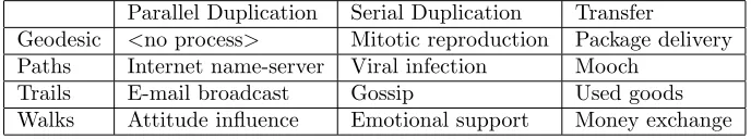
Table 1: The table was originally created by Borgatti (2005), which describes the different network types with a real world example.
Parallel Duplication Serial Duplication Transfer
Geodesic <no process> Mitotic reproduction Package delivery Paths Internet name-server Viral infection Mooch
Trails E-mail broadcast Gossip Used goods
Walks Attitude influence Emotional support Money exchange
3
Measures of Network
Centrality measure has been considered as an attribute of an actor’s position in the network, measurable without regard to how it is connected to others and who and, in turn, how these others are positioned in the network. According to Freeman (1978): ”There is certainly no unanimity on exactly what centrality is or on its conceptual foundations, and there is little agreement on the proper pro-cedure for its measurement. Similarly, Borgatti and Everett (2006) also stated that there is no uniform understanding of an actors central network. There is, however, some very different context-specific interpretations of node centrality which may be the result of the different objectives for the use of centrality mea-sures. These authors posited that determining the centrality of a network is not bounded to one specific measure. Instead, Centrality can be calculated in numerous ways, which depends entirely on the objectives of the search. Further-more, there is a major distinction between finding one central node and finding a set of central nodes. Borgatti and Everett (2006) argued that the problem of getting an optimal set of k-players is different from the problem of selecting kindividuals that are each, individually optimal. This insight originated from the fact that a network may contain multiple nodes that in spite of not having a high degree, have a greater impact in disrupting the network structure when removed (Ortiz-Arroyo and Hussain, 2008).
3.1
Centrality measures for a key player
3.1.1 Degree
Degree Centrality (DC) is a type of radial centrality measure that counts the number of edges a node is attached to. For comparison purposes, DC must be standardized by dividing by the maximum possible value n−1
. The rule is, the node with the highest DC value is the most central node.
DC is one of the easiest measures. It is also considered as a highly effective measure. In many social settings, the people with more connections tend to have more power and more visible. Moreover, the nodes with high degree hold the network cluster together. It is an appropriate measure for the walk-based transfer processes due to the fact that the proportion of times a node is visited is degree dependent (Borgatti, 2005). Nieminen (1974) considered DC as an in-dicator for determining the interconnectedness of a network member. Landherr et al. (2010) had a different view of such matter. They argued that DC does not sufficiently differentiate the interconnectedness of individual member as it only considers the number of immediate contacts but does not consider their further interconnectedness.
3.1.2 Closeness
Closeness centrality (CC) measures the average distance of a node to all other nodes in the network. Scientifically, CC is denoted as:
closeness v
= Pn 1
i=1,i6=vd v, i
(1)
The equation above sums up all the distances of nodev, thed v, irefers to the number of the distance of 1 from the nodev to the nodei. For comparison purposes, CC must be standardized by dividing the maximum possible value of
1
n−1. The rule is, the node with the highest CC value is on average closest to
all other nodes (central node). CC is considered as a measure of how long it takes for information to spread from a source node. It can be applied to both parallel and transfer flows, but it is more accurate when applied to processes that flow along the shortest paths. Both CC and BC neglect network communications that occur along reachable and non-geodesic pathways.
3.1.3 Betweenness
Betweenness centrality (BC) is a type of medial centrality that can be regarded as a measure of the importance of a node as a controller of the information which is flowing between the other nodes in the network. BC measures the number of times a node acts as a bridge along the shortest path (geodesic) between two other nodes. Scientifically, BC is denoted as:
betweenness(v) = X
s6=t6=v
ds,t v
ds,t
The equation above sums up all the all the ratios of (v). (s, t, v) are distinct nodes in the graph, ds,t v
refers to the number of geodesic paths from the node (s) to (t) that via the node v, and ds,t refers to the total number of
geodesic paths from the node (s) to (t). For comparison purposes, BC must be standardized by dividing the number of pairs of nodes that does not includev,
that is, ( n−1
∗ n−2
2 ). The rule is, a node with the highest BC is considered
the most central node.
BC is considered as a measure of volume of traffic moving from each node to every other node that would pass through a given node Borgatti (2005). It is suitable for the transfer types of the process due to its indivisible path that transfers from one node to another along the shortest (geodesic) paths. However, a major downfall with BC and CC is that they do not take into account of flows that are non-geodesic. Furthermore, another problem with BC is in its calculation. De Meo et al. (2012) posited that computing the exact value of BC for each node-edge is almost unfeasible as the graph size grows. Decomposition of the network was considered in avoiding the computational problem, though it will compromise the network infrastructure subtlety.
3.1.4 Other Variations of Betweenness
Due to the limitations of Freemans betweenness, numerous researchers have been building on top of Freemans betweenness over the years and derived various betweenness-like metrics.
3.1.4.1 Flow Betweenness
3.1.4.2 Random-Walk Betweenness
Freemans betweenness measure has the condition that information flowing in the network follows the shortest (or geodesic) paths. However, Estrada et al. (2009) argued that most of the information is likely to flow along non-shortest paths. In this case, the information flow may follow a walk, a trail or a path. In the attempt of overcoming this flaw, Freeman et al. (1991) has introduced flow betweenness centrality which supports both geodesic and non-geodesic paths. However, Newmans finding showed that the flow betweenness was counterintu-itive, which led him to his own alternative concept of random-walk betweenness centrality.
To understand what random-walk betweenness is, it is necessary to under-stand what the definition of random-walk is. Suppose a message that originates at source (s), and it is intended to reach target (t), having no idea where (t) is, simply get passed around until it reaches (t). This means, at each step, the message moves from the current position in the network to one of its adjacent nodes, chosen uniformly at random. Therefore, random-walk betweenness (Noh and Rieger, 2004) is similar to flow betweenness, it measures the frequency of node (v) in between a source node (s) and a target node(t).
The major distinction is that random-walk betweenness is the frequency of node (v) occurring in a random-walk from (s) to (s), whereas flow betweenness comparing the maximum possible paths with paths contain node (v). This distinction provides crucial importance to networks that follow walks trajectory. In the liquid flowing in pipes analogy, the liquid flows in the directions away from the source, thus it is illogical to consider the flow current is in the direction of the source. Unlike trails and paths, walks may contain repeated nodes and edges. When dealing with randomness-walk, it is unlikely that a target node will ever be visited as the size of the network increases. In this case, random-walk betweenness and the betweenness of Freeman (1978) are at the opposite ends of the spectrum (Newman, 2005), where one end represents information has no idea where it is heading and the other end represents information know exactly where it is going. There is one minor yet crucial remark regarding random-walk betweenness. That is, to resolve the biased high betweenness score caused by traversing the same nodes back and forth multiple times, those repeated nodes will be canceled out. Estrada et al. (2009) conducted a simulation on the Strozzi family and correlation analysis on the variety of betweenness measure results. The analysis showed that the lower correlation are observed for the flow betweenness and the shortest path betweenness, whereas the random-walk betweenness exhibited higher correlation (Estrada et al., 2009).
3.1.5 Eigenvector Centrality
same others, they face the same environmental forces and are likely to adapt by becoming increasingly similar. This means that a node is also considered central if it is directly connected to other well-connected nodes. Bonacich (2007) stated that the node that has a high eigenvector score is the one that is adjacent to nodes that are themselves, high scorers. The EC is denoted as:
CE v
∝ X
iN(v)
A v, iCE i
(3)
The equation above sums up all the eigenvector centrality values of neighbors of nodev. CE v
refers to the Eigenvector centrality of nodev,iN(v) refers to nodeibeing one of nodevneighbors, andA v, iCE i
refers to the eigenvector centrality value of nodei.
The mechanism of EC affects all nodes and their neighbors simultaneously, as in a parallel duplication process (Borgatti, 2005). EC does have its limitations, EC neglects multiple shared paths between points that CC and BC do not.
3.1.6 Comparison and Usage
Radial measures are concerned with the position of a node in the network. The direct relationships of a node summarize a node’s connectedness with the rest of the network (Borgatti and Everett, 2006). However, the radial centralities are not suitable in network with multiple dense clusters. Radial centralities make sense in the network which has, at most, one center. Relating to the multiple cluster (two or more centers) networks, medial measures come to play. Unlike radial measures, medial centrality assigns high centrality scores to nodes that serve as a bridge between subgroups (clusters) (Borgatti and Everett, 2006).
When choosing between radial (e.g. DC, EC) and medial (e.g. BC, CC) cen-trality measures, one must consider the conception and cohesion of the network. For example, if one is studying the risk of receiving information flow through the network, then logic dictates that the length measure (medial) would be more suitable. However,if one is studying the package delivery certainty, then the vol-ume measure would be a more obvious choice (Borgatti, 1995). This centrality distinction helps to provide insight into the appropriate centrality measure given the network properties (flow, graph, and transfer mechanism). The previously mentioned centrality metrics from various researchers have been assigned to the network classification developed by Borgatti (2005) according to his research. This is shown in Table 2.
3.2
Diffusion
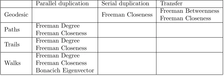
Table 2: The table describes the appropriate centrality metrics for the different network types according to Borgatti (2005).
Parallel duplication Serial duplication Transfer
Geodesic Freeman Closeness Freeman Betweenness
Freeman Closeness
Paths Freeman Degree Freeman Closeness
Trails Freeman Degree Freeman Closeness
Walks
Freeman Degree Freeman Closeness Bonacich Eigenvector
Table 3: The table describes the different factors that contribute toward social influence. These factors are divided into three classes: relational, positional and central)
Relational Positional Central
Direct ties Indirect ties Joint participation
Percent Positive matches: (tie overlap)
Euclidean distance:
(distance between two nodes) Regular equivalence:
(two nodes tie to same 3rd node)
Degree Closeness Betweenness Flow Information Power
social influence processes refer to the number of direct contacts (degree) and position (closeness) of the individual within the network (Burt, 1987). The so-cial influence processes can be modeled with three different classes of network weight matrices (relational, positional, and central) (Table 3). In addition to that, the exposure is also influenced by the social distance and in-degree. For undirected and unweighted networks, the positional and central matrices may be useful in determining the social influence processes. According to Valente (1996), an accelerated diffusion is dependent on the network structure. Diffu-sion reaches pockets of interconnectivity (within the cluster) and spreads rapidly within these pockets, but slow between network subgroups (between clusters). Based on that remark, a starting node that yields the quickest diffusion may be considered as a central source. With that being said, the centrality of the replication processes can be determined by comparing the time needed to reach full diffusion of all nodes.
3.3
Centrality measures for a set of key players
(KPP-Neg) goal consists of identifying those k-players that, if removed, will disrupt or fragment the network. In tackling the Key player problem, Ortiz-Arroyo and Hussain (2008) have developed a method that is based on the en-tropy concept by Shannon (1948). Enen-tropy is defined as a measure to quantify the amount of information that could be transmitted in a noisy communication channel. The basic idea is to find those nodes that produce the largest changes in the connectivity and/or the centrality entropy when removed from the graph.
X v= deg vi
2N (4)
The equation above measures the connectivity of nodev, wheredeg vi
refers to the number of edges attached to nodeVi, andN refers to the total number
of nodes in the network.
Y v
= paths vi
paths v1, v2, v3...vm
(5)
The equation above measures the centrality probability of nodev, wherepaths vi
refers to the number of paths from nodevito all other nodes, andpaths v1, v2, v3...vm
refers to all the paths exist in the networks.
These two equations are used to obtain the different entropy measures (Hco
andHce), by modifying the entropy equation of Shannon (1948). Connectivity
entropy measure (Hco):
Hco G
=−
n
X
i=0
X vi
∗Log2X vi
(6)
Centrality entropy measure (Hce):
Hce G
=−
n
X
i=0
Y vi
∗Log2Y vi
(7)
These two derived entropy equations (Hco G
and Hce G
) help to deter-mine the impact of a node in the graph before and after the removal of that node.
Connectivity entropy measure (Hco G
) determines the degree of connect-edness of a node within the network. In a fully connected graph, the removal of a node will result in a decrease in the total entropy of the graph, in the same proportion as if any other node is removed. However, in a less connected graph, the removal of a node with many incident edges will have a greater impact on the total connectivity entropy of the system, compared to a node with a smaller connectivity degree.
Centrality entropy measure (Hce G) determines the degree of centrality of
The simulation model based on the Algorithm 1 of Ortiz-Arroyo and Hussain (2008) has proven to be a simple yet effective method. Furthermore, It also revealed that the entropy method also identifies redundant nodes in the network.
Algorithm 1: The algorithm describes the machine code of calculating the importance of each node and returns a set of nodes that exceed certain significance level(d1,d2).
Calculate initial total entropy Hco0(G) and Hce0 (G); for all nodes in graph G do:
Remove node vi, creating a modified graph G;
Recalculate Hcoi(G) and Hcei (G), store these results; Restore original graph;
end for;
To solve the KPP-Pos problem select those nodes where Hco0 - Hcoi>d1;
To solve the KPP-Neg problem select those nodes where Hce0 - Hcei>d2;
4
Network
4.1
Information Flow
The centrality measures determine the central players in the network but do not provide much insight regarding the information flow of the network. In the research of Granovetter (1973), the strength of a relationship (tie) is dependent on four components: the frequency of contact, the history of the relationship, the contact duration, and the number of transactions. Granovetter (1973) ob-served that as the frequency of interactions between two people increases, their sentiment of the relationship becomes stronger. The history of the relationship also determines which tie is selected. In a given context environment, a contact with which a person has interacted over a longer period of time may be more important than a newly formed contact. The contact duration and the num-ber of transactions refer to the interaction recency. Granovetter (1973) believes that recency may influence the intensity of the relationship between two people. These indicators can be used for information flow to determine which contact has the strongest social relationship from origin to destination. Tie strength theory provides insight into how information flows in a socio-network. Daly and Haahr (2009) hypothesized that tie strength is a good measure of whether a tie will be chosen or not. Since strong ties are typically more readily available and as result, more frequent interactions may occur. However, unlike strong ties, connecting to a weak tie has its own benefit. The connection to a weak tie enables the access of that circle (subgroup with their own strong ties).
2010). There are three drawbacks associated with the measure of network per-formance that is based on (Zio and Piccinelli, 2010):
1. Binary links (link or no link) in the network, which neglects the strength of the connection. This has been pointed out as a limitation in both social and engineering networks. Zio and Piccinelli (2010) believe that the strength of the interpersonal relationship is relevant in path selection decision.
2. The simplified representation of the social network assumes information flow along the shortest path (geodesic). Based on the context of the in-formation flow, it is very much possible that inin-formation will take a more circuitous route.
3. The simplified representation of the network also neglects the possibility of failure in the interconnection of linked nodes. This could be an associate that is no longer available and it is not been informed to anyone. However, this is particularly relevant for the engineering network that is made of fallible hardware and software.
4.2
Network Structure Properties
Different networks come in different shapes and sizes, each has its unique fea-tures that impacts the information flow. Guzman et al. (2014) have captured three aspects of network structural properties: size, scale-free parameter and clustering coefficient.
4.2.1 Size
Size refers to the number of nodes within a network; the size of a network is context specific. The level of detail determines what actors should be included in the network. The size of the network dictates what the centrality measure is appropriate. For instance, as size increases, it is unwise to use Freemans betweenness due to the scaling of the computational power required.
4.2.2 Scale-free Parameter
Scale-free networks are centralized structure networks with very few dominant nodes. The degree of nodes in such a network follows a power law distribution (1
x2). A power law distribution does not have a peak, instead, it is described
4.2.3 Clustering coefficient
Clustering refers to the grouping of nodes in a network. In a realistic environ-ment, a social network is not centralized. In fact, they are formed by many subgroups each with a significant actor in the middle that is bridged with other subgroups in a larger network. As for this reason, various betweenness mea-sures are more suitable in determining the central nodes in this type of network. However, this is not the case for all types of network. For instance, Freemans closeness centrality is more suitable for the networks that have one cohesive cluster.
4.3
Network Structure
According to Daly and Haahr (2009), Freemans centrality metrics are based on the analysis of a complete and bounded network, which is sometimes referred to as a socio-centric network. However, these metrics become difficult to evaluate when the network size scales up as they require a complete knowledge of the network topology. Due to this reason, the Ego-Network were created. The Ego-Network analysis can be performed locally without the need of complete network knowledge. Alongside Ego-network, other types of network were also introduced. These networks differ in the structural properties that consequently affect information flow drastically.
4.3.1 Ego Network
In an Ego-network (Figure 1) setting by Burt (1987) with equal nodes (ties), dif-ferent information flow outcomes were discovered. In his discovery, two premises were established:
1. People connected by strong ties (by a specific criterion) are considered similar and tend to overlap (e.g. personality, mentality, etc.) (McPherson et al., 2001). Example, the idea generation of two people that are con-nected by a strong tie are more comparable than the idea generation of two people that are connected by a weak tie.
2. People that are connected by the bridge ties (weak ties) tend to spark novel ideas. The benefit of the bridge ties enables the access of other dense groups (groups with their own strong ties).
Figure 2: Exchange Network (Borgatti and Halgin, 2011): The figure displays two versions of the exchange network. The different between the two structures has resulted in the power and centrality difference.
information received at any given time than the structure on the left. Weak ties can be very useful in some settings, they provide bridge connections between different network clusters, allowing subgroups to share access and capabilities (Enriquez, 2010). Granovetter (1973) emphasized that the weak ties can lead to information dissemination between groups. He stated that information can reach a large number of people and traverse a greater social distance when passes through weak ties rather than strong ties. In addition to that, weak ties also provide people with access to information and resources beyond those available in their own social cluster.
4.3.2 Exchange Network
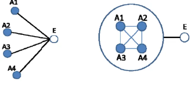
Figure 3: Unionization Network (Borgatti and Halgin, 2011): The figure displays how similar nodes in a network can be interpreted as on unit.
weak (Willer, 1992).
4.3.3 Unionization Network
Consider a network setting (Figure 3) in which multiple of similar actors (A1, A2, A3, and A4) in communication with one other actor (E). Like in a factory with multiple low-level workers, who report to the same supervisor. Reporting to the same supervisor individually can be time-consuming and difficult. The principle of unionization is that if multiple actors have similar goals, then they can be treated as one unit. The key point in a unionized network is that nodes with the same interests and capabilities working together can accomplish more than they could alone. This is the so-called ”network organization”, in which a set of autonomous unit coordinate closely as if comprising a single, superordinate entity (Powell, 2003). The bonding function between the actors is called bond model which is the analog of the flow function in the flow model.
4.4
Random Network vs. Scale-free Network
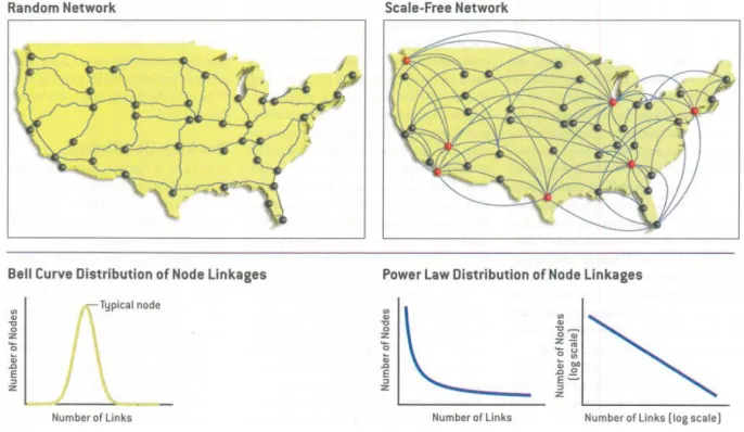
Figure 4: Random vs. Scale-free Network (Barab´asi and Bonabeau, 2003): The simplified highway intersections of US is shown on the left. The simplified US airline on the right. They correspond to the specific type of network shown in the figure.
number of connections to neighbor states. In this example, it is indeed rare to find interactions with fewer and/or many connections. As for the scale-free network, the links of nodes in the network follow the power-law distribution, which is the probability of a node connecting tok other nodes is proportional to k1n. A scale-free network has an abundant of nodes with fewer links and few nodes with high links. A node with many connections in a scale-free network is called a hub. Networks with central hubs are robust against accidental failure, but vulnerable to coordinated attack (fragility) (Grassi, 2010). Understanding such characteristic is vital to the development of centrality metrics for parallel and serial replication. Few life examples of a scale-free network are the Swedish sexual relationship, while many people have few sexual partners, a few had hundreds in their lifetime. Published scientific papers with citations, Internet systems with routers and the World Wide Web with web pages are examples of the power-law network.
literature stimulate even more researchers to read and cite them, a phenomenon that noted sociologist Robert K. Merton called the Matthew effect, after a pas-sage in the New Testament: ”For unto every one that hath shall be given, and he shall have abundance.” These two reason help to explain the existence of hubs and help in the construction of networks.
4.5
Cohesion and Clustering
Since all the networks are not identically shaped. The question is, at what point a network is considered as a cohesive group or a multiple cohesive subgroups (clustering) network? One of the first intuitions in SNA concerns the tendency of human beings to form cohesive subgroups. The main characteristic is that the nodes in a subgroup are similar in attributes. People adjust their behavior and attitudes, opinions, and beliefs to the behavior of other members of the social system in which they participate. Over time, people decide on which ties to establish, maintain, or terminate (social selection model). The key player set theory (Ortiz-Arroyo and Hussain, 2008) suggests that some networks have multiple vital players. These key players may hold some strong positions in the network. In such case, how would one determine the cohesive subgroups in a network? The clustering coefficient (CCoe) of the network determines how cohesive the nodes in the network are. The measure of CCoe is based on the triplet of nodes. A triplet is three nodes that are connected to each other forming a triangle. The global clustering coefficient is the average of triplet ratios of all the nodes. The end result is a value from a scale between 0 and 1. The networks with low CCoe value are structured like a star shape (hub - like), whereas the networks with high CCoe value are structured like a clique (close-knit group).
5
Development of Centrality Metrics
The in-depth knowledge of the network structures and their unique character-istics along with a variety of centrality measures from the previous chapters provided a solid foundation in the formulation of suitable centrality approaches for other network types. With that being said, this chapter is aimed at develop-ing appropriate methods accorddevelop-ing to the network examples of Borgatti (2005) (Figure 1).
5.1
Centrality
Centrality is an abstract property of a nodes position in a network (Enriquez, 2010). Centrality corresponds to the overall network property and it is defined as the variation of centrality scores of all nodes. The variation of centrality scores describes where the central nodes and/or peripheries are. The star and ring networks are considered respectively the most and the least centralized networks (Borgatti et al., 2009). The fundamental metrics (Degree, Closeness, Betweenness, Eigenvector Centrality) are not applicable to all types of network flow. Degree and Eigenvector metrics focus on the immediate relationships. Both Betweenness and Closeness are based on the idea of information flow along the shortest path (Freeman, 2004). There are other networks in which infor-mation does not flow along the geodesic path (Stephenson and Zelen, 1989). News, rumors or messages do not know the ideal route to take. They simply moves from one place to another; more likely it wanders around more randomly (Newman, 2005). The random-walk betweenness approach of Newman (2005) and flow betweenness approach of Freeman et al. (1991) are promising solutions in addressing such problem. Despite all that, there is another concern regard-ing what centrality metrics are appropriate for the network with different flow mechanisms (parallel, serial and/or transfer). In the example of a viral infec-tion (Path - Serial duplicainfec-tion) that virus spreads around randomly, infecting one person at a time. Determining the centrality of a single node in the net-work using conventional metrics may not yield useful results. Instead, it may be wise to inspect such phenomenon differently. The work of key player set by Borgatti (2006) mentioned in the earlier chapter determines the centralization of the network by weighing the importance of each node, neglecting the flow mechanism. Furthermore, the key player set may also be used as a validation tool in determining the reliability and validity of the proposed methods.
5.2
Formulation of Methods
state of the information does not vary under any circumstances. For instance, the condition of the used good (example by Borgatti (2005) ) that is passing around within the network does not change over time.
5.2.1 Serial and Parallel Replication
In the scenario of serial and parallel duplication, it would take some time to reach full diffusion starting from sourceS and end at multiple targets T s. Assuming the information spread takes place in incremental steps, then the number of reached nodes after each intermediate incremental step is an addition to the current step. At some point in time, all the nodes will have a copy of the information that was transmitted from the sourceS. Based on this premise, the nodes require the least amount of time to reach full diffusion would be considered as central (definition of centrality). This idea is based on Freemans closeness centrality, flow betweenness and key player set (Borgatti et al., 2009; Ortiz-Arroyo and Hussain, 2008). Freemans closeness was discovered to determine the centrality of a geodesic transfer network. Instead of closeness based on geodesic paths, all possible paths should be taken into account (flow betweenness). The main objective is to find a suitable source position (central node), such that the minimal time interval is needed to reach full diffusion (Iribarren and Moro, 2011; Valente, 1996; Burt, 1987).
5.2.1.1 Serial: Paths
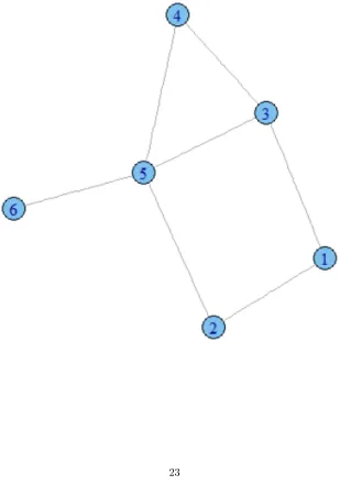
In a serial duplication, only one copy of the information per node is replicated per time. For path trajectories, each of the possible adjacent neighbors of a node is a potential receiver of the replication which means that each selection of a receiver leads to a completely different path. Let’s use the viral infection example (Figure 1) by Borgatti (2005), a person (node) cannot infect someone who has already been infected (already received a copy of the virus) or someone who he received the virus from. At each time interval, the maximum number of possible virus infections (number of copies) is equal to the number of infected people. This virus spreads until all the people in the network are infected (all the people received a copy of the virus). The proposed approach is a closeness-like measure (Borgatti and Everett, 2006), which assesses the length of the walks that a node is involved in.
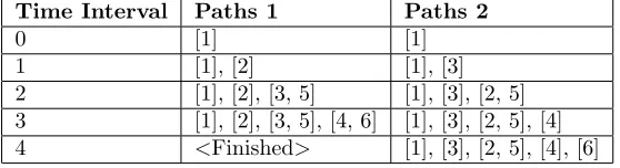
Table 4: The table described the spread of the virus based on the Simple Net-work Example (Figure 5). The table contains two of many possible diffusions with person 1 as the source. During each time interval, newly infected people are appended.
Time Interval Paths 1 Paths 2
0 [1] [1]
1 [1], [2] [1], [3]
2 [1], [2], [3, 5] [1], [3], [2, 5]
3 [1], [2], [3, 5], [4, 6] [1], [3], [2, 5], [4] 4 <Finished> [1], [3], [2, 5], [4], [6]
in 3-time intervals. However, if the virus replication had taken a different path (Table 4: Path 2), atT I = 3, only person 3 and person 5 could have the possi-bility to spread the virus. If person 5 infects person 4, then the last person in this small network (person 6) can only be infected by person 5 in the next time interval (T I= 4). In such case, the virus diffusion took 4-time intervals. Since there are countless virus diffusion possibilities, the only way to obtain a plausi-ble measure is by taking the average score of many runs. In this brief example, 2 runs (Path1 and Path 2) were mentioned, thus the average centrality value of person 1 is 3.5 ((3 + 4)/2 = 3.5). This procedure is applied to all other nodes in the network to determine which nodes are the most central. The workings of the example above are translated into machine code (Algorithm 2).
Algorithm 2:The algorithm represents the machine code that is used to determine the serial-paths centrality value of each node in the network.
Iterate over simulation runs:
Create an empty queue to to store all possible paths combinations; Store the first node;
While queue is not empty:
Get first path sequence from the queue;
Iterate over the neighbors of each node in the path sequence: Store one neighbor node if not been visited to a temporary list; If the temporary list is not empty:
Create new possible path sequence and add it to queue; Else:
Determine and add length of current path sequence; Determine average time interval of a node;
5.2.1.2 Serial: Trails
be repeated but the edges cannot. Lets use the example of gossip by Borgatti (2005), a person (A) can tell a rumor to person (B) in a gossip, even though person (B) has already heard it from person (D). But, person (B) cannot tell that very same rumor back to person (D) or person (A). This unique property may impact the course of gossip spread. Instead of picking a person who is not aware of the rumor, picking someone who may have heard of the rumor is entirely possible. This results in more node selection possibilities and thus longer time needed to reach full diffusion.
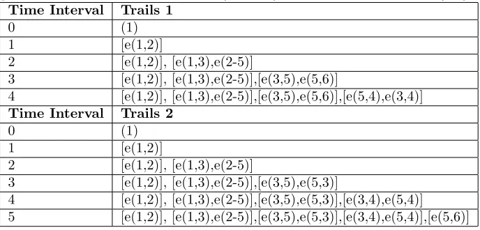
Table 5: The table describes the spread of a rumor in a gossip based on the Simple Network Example (Figure 5). The table describes two possible rumor diffusions with person 1 as the source. During each time interval, the newly gossip occurred between two people (a and b) are described in form of e(a,b).
Time Interval Trails 1
0 (1)
1 [e(1,2)]
2 [e(1,2)], [e(1,3),e(2-5)]
3 [e(1,2)], [e(1,3),e(2-5)],[e(3,5),e(5,6)]
4 [e(1,2)], [e(1,3),e(2-5)],[e(3,5),e(5,6)],[e(5,4),e(3,4)]
Time Interval Trails 2
0 (1)
1 [e(1,2)]
2 [e(1,2)], [e(1,3),e(2-5)]
3 [e(1,2)], [e(1,3),e(2-5)],[e(3,5),e(5,3)]
4 [e(1,2)], [e(1,3),e(2-5)],[e(3,5),e(5,3)],[e(3,4),e(5,4)] 5 [e(1,2)], [e(1,3),e(2-5)],[e(3,5),e(5,3)],[e(3,4),e(5,4)],[e(5,6)]
Assuming both gossip diffusions (Table 5: Trails 1 and Trails 2) occurred the same priorT I = 3, the random gossip partner selection have led to different outcomes. In Trails 1, assuming during T I = 3, person 3 and person 5 have selected person 5 and person 6 respectively, then the remaining person (person 4) would have to be picked by either person 5 or 3 in the next time interval (T I = 4). In comparison to Trails 2, the gossip partner selection fromT I = 3 had led to a different diffusion outcome. Due to person 3 and person 5 had selected each other inT I = 3, this resulted in an additional turn in completing the rumor diffusion (T I = 5). Similar to serial paths, there are countless ways in which how the diffusion could have progressed. Thus,it is a must to take the average score of all the runs. In this particular example, the average centrality score for person 1 is 4.5 ((4 + 5)/2 = 4.5). This procedure is applied to all other nodes in the network to determine which nodes are the most central. The workings of the example above are translated into machine code (Algorithm 3).
Algorithm 3:The algorithm represents the machine code that is used to determine the serial-trails centrality value of each node in the network.
For every node in th network: Iterate over simulation runs:
Create an empty queue to to store all possible paths combinations; Store the first node;
While queue is not empty:
Get first path sequence from the queue;
Iterate over the neighbors of each node in the path sequence: Form new edge with node and its neighbors;
Store the neighbor node if newly formed edge is not in temporary list; If the temporary list is not empty:
Create new possible path sequence and add it to queue; Else:
Determine and add length of current path sequence; Determine average time interval of a node;
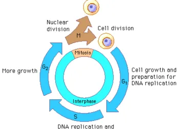
Serial geodesic is uniquely different from paths and trails. A real-world example of such network is a mitotic reproduction (Figure 6) thought by Borgatti (2005), where a cell divides into two at each iteration (i.e. 1 becomes 2, 2 become 4, so on and so forth). One would consider this manifestation behavior like a tree structure with 2 children at each level. At the nth level, the number of children is equal to 2n. Based on the analogy of mitotic reproduction, the total
number of cells that can reproduce at a time interval (TI) is the twice of a total number of cells in the previous time interval (TI - 1). Using the network example (Figure 5), each node represents a possible cell with its unique traits, and each edge represents the potential of producing cells with a specific mutation. For example, cell 5 (node 5) has the potential to produce cells 2, 3, 4 and 6. However, cell 1 can only be produced by either cell 2 or 3. In this particular scenario, a geodesic serial replication can be interpreted as the shortest time needed to produce a full range of cells with different traits. This is only possible by possible by maximizing the number of newly produced cells during each time interval. such that the total number of replications is maximized. With that being said, the starting cell that is able to produce a full range of cell with the least amount of time is considered the most important cell (central node).
Table 6: The table described the mitotic reproduction based on the network (Figure 5), and with parent cell 1 (node 1). It maximizes the production of the distinct cell during each iteration.
Time Interval Geodesic
0 [1]
1 [1], [2]
2 [1], [2], [3, 5]
3 [1], [2], [3, 5], [4, 6]
4 <Finished>
which parent cells are able to produce a large variety of cell traits in the least amount of time. This is achieved by determining the cell with minimal time interval needed to produce a wide range of distinct cells for each source cell. The above-mentioned approach is translated into machine code (Algorithm 4).
Algorithm 4:The algorithm represents the machine code that is used to determine the serial-geodesic centrality value of each node in the network.
For every node in the network: Iterate over simulation runs:
Create an empty queue to store all possible path combinations; Store first node;
While the queue is not empty:
Get first path sequence from queue;
Iterate over the neighbors of each node in the path sequence; Store nodes that have not been visited in a temporary list; Sort temporary list according to minimal remaining neighbors; While temporary list is not empty:
Get first node from list, and add to addOn list; Remove node from the temporary list;
Loop over every node in the temporary list is account for; If addOn list is not empty:
Create new path sequence with nodes in addOn list; Else:
Add up all the path sequences lengths; Determine average time interval of a node;
5.2.1.4 Parallel: Paths and Trails
paths and trails of a parallel replication differs in the number of replications of information a node receives, there is no difference in terms of time needed to reach full diffusion. The nodes of trails may have multiple copies of the information. In the example of Email broadcast, Email is sent from source (S) and are received by multiple recipients (Rs) at each time interval. In the next time interval, the recipients who have already gotten that email may receive receive another copy from another sender. Borgatti (2005) proposed Freemans degree and closeness to measure centrality for paths, trails, and walks. The time step approach similar to Freemans closeness centrality, which determines the network centrality by finding the node that is closest to all other nodes.
Table 7: The table describes the email broadcast based on the Simple Network Example (Figure 5). The table describes 2 possible email broadcasts with dif-ferent points of origin. During each time interval, the new recipients appended.
Time Interval Paths / Trails 1 Paths /Trails 2
0 [5] [1]
1 [5], [2, 3, 4, 6] [1], [2, 3]
2 [5], [2, 3, 4, 6], [1] [1], [2, 3], [4, 5] 3 <Finished> [1], [2, 3], [4, 5], [6]
The two parallel replication processes with different source nodes yielded different results. The parallel replication example (Table 7) showed that the broadcast with source sender 5 took 2-time intervals (T I= 2), while the broad-cast with source sender 1 needed 3 (T I = 3). Since all the nodes simultaneously received a copy of the replication, there is no need to conduct multiple runs. The above-mentioned approach is translated into machine code (Algorithm 5).
Algorithm 5:The algorithm represents the machine code that is used to determine the parallel - paths and/or trails centrality value of each node in the network.
For every node in the network:
Create an empty queue to store all possible path combinations; Store first node;
While the queue is not empty:
Get first path sequence from queue;
Iterate over the neighbors of each node in the path sequence; Store the nodes that have not been visited in a temporary list; While temporary list is not empty:
Create new path sequence with the nodes in temporary list; Else:
5.2.2 Transfer
As for the transfer mechanism, measuring centrality for geodesic, paths, trails, and walks would not work with the approach designed for serial and/or par-allel replication. Because the transfer mechanism states that the information is passed onto the adjacent node without leaving a copy. Furthermore, the concept of diffusion does not apply in the networks with transfer mechanism. One possible way to determine centrality is by looking at how much each node has contributed to the transfer flow. Of course, there are four types of trans-fer mechanisms: geodesic, trails, paths, and walks. Each of them is uniquely different and thus a custom-made approach for each of them is a must. The centrality metrics for the geodesic types already existed. Freemans between-ness and closebetween-ness centrality are specifically designed for geodesic flows. With that being said, the following proposed approaches are aimed at other types of transfer process.
5.2.2.1 Transfer: Paths
Freemans closeness and betweenness are designed to measure geodesic (i.e. pack-age delivery). With packpack-age delivery example, the assumption is that the short-est route is known and chosen, while paths (i.e. mooch) takes a random path. Based on that premise, an effective approach in measuring centrality is by deter-mining the involvement of the nodes. The proposed approach is a betweenness-like measure (Borgatti and Everett, 2006), which measures the number of walks that passes through a given node. In a transfer paths flow, with starting node (S) and target node (T), the set of nodes that have been traversed would be counted as nodes in between (S) and (T). Since there are multiple nodes in the network, picking a fixed starting point and ending point would produce bias results. Therefore, every single combination of size 2 nodes (start and target) must undergo the same process. The centrality measure of a node (I) is equal to the number of different paths that node (I) is involved in. Since a node is chosen at random during each traverse and not possible for a node to be visited twice, it is unlikely that all the possible information flow combinations can be achieved. Therefore, the in-between nodes of the incomplete paths (unable to each target node from start) are excluded. At the end of all information flow combinations, the centrality measure node (I) is the ratio of node occurrence and flow combi-nation size. The node that has the highest proposed betweenness-like value is considered as the most central node.
Table 8: The table describes the mooch between people based on the Simple Network Example (Figure 5). The flow combination column represents the starting and ending person of the mooch event. The transfer paths column shows all the intermediate people that have been asked for favors. The between nodes column displays all people who were in between the starting person and ending person.
Flow Combination Transfer Paths Between Nodes
[1, 2] [1], [3], [5], [2] [3], [5]
[1, 3] [1], [3]
-[1, 4] [1], [2], [5], [6]
-...
2 [1,3] is rejected due to no in-between node, and flow combination 3 [1,4] is rejected due to the requirement of ending at node 4 is not met. So, based on this particular example, the transfer paths centrality measure for both person 3 and person 5 is n1 (1 occurrence in n different flow combinations). The above-mentioned approach is translated into machine code (Algorithm 6).
Algorithm 6:The algorithm represents the machine code that is used to determine the transfer - paths centrality value of each node in the network.
Get all (start, end) tuples in a list; Iterate over simulations runs: Iterate over all (start, end) tuples:
Create an empty list to store nodes; Add the start node in the list; While:
Get last node from the list;
Pick a neighbor that has not been visited randomly; If last node is end node:
Terminate;
If last of the list is end node: Count each in-between node; Iterate over all the nodes in the network:
Determine average result of a node;
5.2.2.2 Transfer: Trails
repeated, reaching the target node from the starting node is more feasible. On the other hand, the repeated nodes property also increases the node selection pool and thus, it is highly likely that the size of in-between nodes of trails is much larger than the size of in-between nodes of paths. The centrality measure of a node is the ratio of the node occurrence and the flow combinations.
Table 9: The table describes the transfer of a used good between people based on the Simple Network Example (Figure 5). The flow combination column represents the starting person and the ending person of the used good transfer. The transfer trails column shows all the transfers between two people in the form ofe(a, b). The between nodes column displays all people who were in-between the starting person and the ending person.
Flow Combination Transfer Trails Between Nodes
[1, 6] [e(1,2), e(2,5), e(5,4), e(4,3), e(3,5), e(5,6)] [2, 5, 4,3, 5] ...
Consider the used goods example by Borgatti (2005). The passing of the used good (Table 9) strictly showed that no edges can be repeated. Since once you have passed the used good onto another person, it is unlikely that you want it back. Though, you may accept the used good if it was originating from another person. The above example (Table 9) showed that person 5 is has accepted the same used good twice, but by from two different people (person 2 and person 3), thus it is completely acceptable. The occurrence of each in-between person is stored. In this case, the occurrence of person 5 is counted twice. Once all the different flow combinations have been processed, the average occurrence is the total occurrence (Ot) of each person divided by the total number of flow
combinations (Ot
n ). The above-mentioned approach is translated into machine
code (Algorithm 7).
5.2.2.3 Transfer: Walks
Algorithm 7:The algorithm represents the machine code that is used to determine the transfer - trails centrality value of each node in the network.
Get all (start, end) tuples in a list; Iterate over simulations runs: Iterate over all (start, end) tuples:
Create an empty list to store nodes; Add the start node in the list; While:
Get last node from the list;
Create new edge with last node and one random neighbor node; Add node, if new edge not yet visited;
If last node is end node: Terminate;
If last of the list is end node: Count each in-between node; Iterate over all the nodes in the network:
Determine average result of a node;
[image:33.612.140.477.151.341.2]forth are neglected.
Table 10: The table describes the money exchange between people based on the Simple Network Example (Figure 5). The flow combination column represents the starting and ending person of the money exchange. The walks sequence before shows all the intermediate people involved in the money exchange. The walks sequence after removes any ’back and forth exchanges’ between two peo-ple.
Case Flow Combination Walks Sequence Before Walks Sequence After
1 [1, 6] [1, 2, 5, 4, 5, 6] [1, 2, 5, 6]
2 [1, 6] [1, 2, 5, 4, 3, 5, 6] [1, 2, 5, 4, 3, 5, 6]
...
tween node. Once all the flow combinations have been processed, the node with the highest ratio is considered as the most central node. The above-mentioned approach is translated into machine code (Algorithm 8).
Algorithm 8:The algorithm represents the machine code that is used to determine the transfer - walks centrality value of each node in the network.
Get all (start, end) tuples in a list; Iterate over simulations runs: Iterate over all (start, end) tuples:
Create an empty list to store nodes; Add the start node in the list; While:
Get last node from the list;
Randomly pick a neighbor node of the last node; If picked node is the same as second last node:
Remove last two nodes Else:
Add node to list; If last node is end node:
Terminate;
If last of the list is end node: Count each in-between node; Iterate over all the nodes in the network:
Determine average result of a node;
6
Realization
In order to determine the validity and reliability of the proposed methods for measuring different types of network process, a stable simulation environment is needed. The simulation environment includes the basis of the network with dynamic network property input (size, power-coefficient, cluster, etc), and the different measures that were mentioned in the previous chapter. The construc-tion of the simulaconstruc-tion is based on Python programming language on Spyder IDE with few imported libraries which will be mentioned later in this chap-ter. Python is chosen due to the capability of processing large data set, and the marvelous built-in functions, all of which may contribute greatly to this research.
6.1
Construction of Network
user-defined attributes (Table 11). Object-oriented programming (OO) is se-lected over the adjacency matrix, simply because OO is more flexible with the future modifications and scaling. The different variables within the Node class store the centrality measures and other relevant data. Once the class is con-structed, the next step is to create nodes and forming edges that comply with different network types (random or scale-free) and different network properties (size, power-parameter, clustering coefficient).
Table 11: The tables describes all the relevant attributes of each node object. The attributes include a set of neighboring nodes, variables to store different centrality measures and node identifier.
Class: Node
Variable Data Type
id string
links Integer
neighbors list
degree float
closeness float
betweenness float
eigenvector float
Transfer Paths float
Transfer Trails float
Transfer Walks float
closeness Serial Geodesic float closeness Serial Paths float closeness Serial Trails float closeness Parallel Paths float
6.1.1 Creation of Nodes and Formation of Edges
the chosen node must have free links and it is not linked with the node. With scale-free, the selection of node is not random, instead, it follows the concept of preferential selection or ’The Rich gets Richer’ analogy. The preferential selec-tion states that a node is more likely to form a connecselec-tion with nodes that have a higher connection. This phenomenon is why Barab´asi and Bonabeau (2003) referred to it as The Rich gets Richer. Similar to random, the chosen node must not violate the conditions.
Algorithm 9:The algorithm represents the machine code that is used to construct node according to random and/or scale-free network.
If random network:
Get random linkage distribution and store them in a linkage list; Iterate over network size:
Create new node with specific amount of links; Pick a random node from the existing network; If chosen node neighbor is not full:
Form connection with chosen node; Add this new node to the network; Else if scale free network:
Get power law linkage distribution and store them in a linkage list; Sort linkage list, descending order;
Iterate over network size:
Create new node with specific amount of links; Choose a random node based on links of the node; If chosen node neighbor not full:
Form connection with the chosen node; Add this new node to the network;
The machine code (Algorithm 9) (Algorithm 10) are capable of specifying network property parameters (size and power-law parameter). However, it is not possible to specify the cluster, but it is possible to determine the clustering coefficient of the network. All of which will come in handy when conducting the simulation studies. The clustering coefficient is built based on the working prin-ciple of triangle formations in the A Clustering Coefficient Network Formation Game by Brautbar and Kearns (2011). It is determined by taking the average of the triangle-degree ratio of all the nodes (See Algorithm 11).
6.2
Construction of Centrality Metrics
Algorithm 10:The algorithm represents the machine code that is used to establish connections among nodes.
Iterate over every node in the network:
Store nodes that need neighbors in the possible list; While current node has free neighbor slot:
If possible list is not empty:
Choose a random node from the possible list; If chosen node and current node are not neighbor:
Form connection between the two nodes; Else:
Remove chosen node from possible list; Else:
Choose a random node from the entire network; If chosen node and current node are not neighbors:
Form connection between the two nodes;
node object, which was vital to the non-geodesic simulation scenarios. For each specific Python code, see Appendix: Python Core Code.
7
Simulation Study
A simulation study is an experiment that is conducted on a small representation of the real world setting. A simulation study is often applied in practice as the main benefit of the simulation study is cost saving. Depending on the type of experiment, live testing can be expensive and maybe not feasible. The simulation study is capable of producing a high volume of reliable results that may be difficult to achieve in real-world testing. These difficulties stem from time, ethics and other practical reasons (Bandini et al., 2009). Generally, a simulation study serves two areas: predictive research and explanatory research (Figure 7). However, there is a crucial factor of a simulation study, that is, how representative is the simulation model? If results are obtained from an unreliable simulation model, then the produced results are rendered useless. Therefore, a validation procedure must be conducted before the simulation can be begin.
7.1
Validation
Algorithm 11:The algorithm represents the machine code that is used to determine the cluster coefficient of the network. CCgraphrefers to the
cluster coefficient of the entire network, whileCCnoderefers triangle ratio
of particular node.
CC graph counter set to 0;
Iterate over all the nodes in the network: CC node counter set to 0;
If node has at least two neighbor nodes: Triangle counter set to 0;
If any node with two other neighbors forms a triangle: Add one to triangle counter;
CC node = triangle/(node neighbors size*(node neighbors size -1)); CC graph += CC node;
CC graph = CC graph/network size;
and Hussain (2008). Ortiz-Arroyo and Hussain (2008) determine the importance of nodes in a network by analyzing the degree of connectivity and centrality of each node in the network. Despite the lack of existing models to compare with, it is possible to validate the proposed measures by comparing their results. If the central nodes produced from the proposed methods are aligned with the results of key players set, then the proposed measures are considered valid. Before applying Ortiz-Arroyo and Hussain (2008) entropy validator on the proposed measures, the validator model should also be validated. The entropy validator will be applied to the proposed centrality measures on the ”Florentine Family” network, once it has been validated.
7.1.1 Validation of the Entropy Validator
To validate the entropy validator, a simple fully connected network of size 5 is constructed. Ortiz-Arroyo and Hussain (2008) state that the removal of any node in a fully connected network will have the same impact (Figure 8).
The graph (Figure 9) refers to the difference of impact each node has on the entire network. The ID of each node is displayed by integers on the x-axis (i.e. 0 on the x-axis is referred to node 0, so on and so forth.) and level of node removal impact is represented by the y-values. It can be seen that the removal of each has an equal amount of influence on the entire network. This finding is in line with the characteristics of a fully connected network. This result indicates that the entropy validator is valid in itself and can thus be used in this research.
7.1.2 Validation of the Proposed Measures
Figure 7: The figure describes the different phases of a traditional simulation study. (Image Source: Bandini et al. (2009))
[image:39.612.150.462.386.708.2]Figure 10: The graph presents the importance of each node of the Florentine family. The individual family represented on the x-axis while y-axis measures the connectivity and centrality entropy.
T able 12: The table describ es the sim ulation results based 100 runs. Eac h c olu m n represen ts differen t cen tralit y measure, the v alues are m easured accordin g to the v arious cen tralit y metrics. Eac h cen tralit y measure has its o w n v alue scale (i.e. V alues of Bet w eenness and Closeness should not b e used in comparison). No de ID En trop y Connectivit y En trop y Cen tralit y P arallel P aths/T rails Serial Geo desic
Serial Paths Serial Trails
[image:42.612.143.383.74.690.2]Table 12 shows the result of all the proposed centrality approaches based on 100 simulation runs. The general finding regarding the top results of each approach is that Medici is the most central node. The parallel and serial du-plication methods incorporates Freemans closeness-like and flow-betweenness principles. As result, Medici, Ridolfi and Tornabuon are the top 3 candidates in the serial and parallel replication rankings. A plausible explanation as to why Ridolfi and Tornabuon do not produce a significant impact in the central-ity entropy and connectivcentral-ity entropy measures, is that the positions of Ridolfi, Tornabuon and even Medici are situated closest to all other nodes. This effect is shown in Figure 10 as the removal of Ridolfi or Tornabuon do not produce a significant impact in reducing the number of viable paths for other nodes. This implies that the absence of one of those nodes will not influence the diffu-sion rate. Furthermore, since Ridolfi and Tornabuon do not have high degree centrality, they do not stand out in the connectivity entropy measure.
The proposed transfer methods are based on the random-walk betweenness, which also produced similar results. The top results of all the transfer ap-proaches are supported by the connectivity entropy measure. Since the infor-mation is immutable and cunreplicated, it exists in one place at any point in time. This means that the nodes that are well connected in the network are more likely to be chosen. Strozzi is the balance between high connectivity and centeredness, he is positioned on the paths of many nodes and the fact that he has high degree centrality makes Strozzi a strong candidate for random node selection. Meanwhile, both Guadagni and Albizzi have high connectivity mea-sure, but they are not considered in the proposed transfer measures. As they are located outside of the core center, making them less accessible.
Based on the findings and analysis above, it is conclusive to say that the proposed methods are well constructed and produced consistent results. This implies that the proposed methods can be used to test the different network property settings.
7.2
Experimentation
In the experimentation phase different centrality measures including the pro-posed ones will be tested on a variety of networks. Guzman et al. (2014) clas-sified network properties into three types: size, power-law parameter, and clus-tering coefficient. Barab´asi and Bonabeau (2003) made a significant distinction between random and scale-free network. Once all the factors have been tested, data analysis will be conducted in the attempt to answer the proposed research questions. The aim of the simulation study is not to produce a predictive result, but rather examine how the centrality measures are influenced by the network properties.
7.2.1 Experiment settings