Dynamics of Almost Periodic Mutualism Model
with Time Delays
Yaqin Li, Lijun Xu, and Tianwei Zhang
Abstract—By using some new analytical techniques, modified inequalities and Mawhin’s continuous theorem of coincidence degree theory, some new sufficient conditions for the existence of positive almost periodic solutions to a mutualism model with bounded and unbounded delays are obtained. Further, the boundedness and global asymptotic stability have been studied. To the best of the author’s knowledge, so far, the result of this paper is completely new. The work of this paper extends and improves some results in recent years. Finally, some examples are given to illustrate the main results in this paper.
Index Terms—Almost periodicity; Coincidence degree; Mu-tualism model; Bounded and unbounded delays.
I. INTRODUCTION
L
Et R, Z and N+ denote the sets of real numbers,integers and positive integers, respectively. Related to a continuous functionf, we use the following notations:
fl= inf
s∈R
f(s), fM = sup
s∈R
f(s),
|f|∞= sup s∈R
|f(s)|, f¯= lim
T→∞
1
T
Z T
0
f(s) ds.
Mutualism, or cooperation, is found in many types of com-munities. For example, some species of Acacia require the ant Pseudomyrmex in order to survive (see [1]), blue-green algae can grow and reproduce in the absence of zooplankton grazers, but growth and reproduction are enhanced by the presence of the zooplankton (see [2]).
In [3], Gopalsamy had proposed the following model to describe the mutualism mechanism:
dN1(t)
dt = r1(t)N1(t)
hK
1(t)+α1(t)N2(t)
1+N2(t) −N1(t)
i
,
dN2(t)
dt = r2(t)N2(t)
hK
2(t)+α2(t)N1(t)
1+N1(t) −N2(t)
i
,(1.1) where ri denotes the intrinsic growth rate of species Ni, i = 1,2. The carrying capacity of species Ni is Ki in the absence of other species, while with the help of the other species, the carrying capacity becomes[Ki+αiN3−i]/[1 + N3−i], i = 1,2. The above mutualism can be classified as facultative, obligate or a combination of both.
Naturally, more realistic and interesting models of popula-tion interacpopula-tions should take into account both the seasonality of the changing environment and the effects of time delay. In system (1.1), the mutualistic or cooperative effects are not realized instantaneously but take place with time delays.
Manuscript received September 19, 2017; revised February 18, 2018. Yaqin Li is with the Department of Mathematics, Kunming University, Yunnan 650214, China. ([email protected]).
Lijun Xu is with the School of Mathematics and Computer Science, Panzhihua University, Panzhihua, Sichuan 617000, China. ([email protected]).
Tianwei Zhang is with the City College, Kunming University of Science and Technology, Kunming 650051, China. ([email protected]).
Correspondence author: Tianwei Zhang. ([email protected]).
Therefore, by way of Mawhin’s continuous theorem of coincidence degree theory, Li [4] investigated the existence of positive periodic solutions for a periodic mutualism model with bounded delays:
dN1(t)
dt = r1(t)N1(t)
K1(t)+α1(t)N2(t−µ2(t))
1+N2(t−µ2(t))
−N1(t−ν1)
,
dN2(t)
dt = r2(t)N2(t)
K2(t)+α2(t)N1(t−µ1(t))
1+N1(t−µ1(t))
−N2(t−ν2)
,
(1.2)
where ri, Ki, αi ∈ C(R,(0,∞)), αi > Ki, µi, νi ∈ C(R,[0,∞)),ri, Ki, αi, µi, νiare functions of periodω >0, i= 1,2.
Next, Li and Xu [5] studied the following model of two species mutualism with unbounded delays:
dN1(t)
dt = r1(t)N1(t)
H1(t)+β1(t)R0∞J2(s)N2(t−s) ds
1+R∞
0 J2(s)N2(t−s) ds
−N1(t−ν1(t))
,
dN2(t)
dt = r2(t)N2(t)
H2(t)+β2(t)
R∞
0 J1(s)N1(t−s) ds
1+R∞
0 J1(s)N1(t−s) ds
−N2(t−ν2(t))
.
(1.3)
Under the assumption that ri, Hi, βi and νi are continu-ous periodic functions with common period ω, ai > Ki, Ji ∈ C([0,∞),[0,∞)) and
R∞
0 Ji(s) ds = 1, i = 1,2, they showed that system (1.3) admits at least one positive ω-periodic solution by way of Mawhin’s continuous theorem of coincidence degree theory.
In real world phenomenon, the environment varies due to the factors such as seasonal effects of weather, food supplies, mating habits, harvesting. So it is usual to assume the periodicity of parameters in the systems. However, if the var-ious constituent components of the temporally nonuniform environment is with incommensurable (nonintegral multiples, see Example 1.1) periods, then one has to consider the environment to be almost periodic [6-12] since there is no a priori reason to expect the existence of periodic solutions. Hence, if we consider the effects of the environmental factors, almost periodicity is sometimes more realistic and more general than periodicity.
Example 1. Let us consider the following simple population
model:
˙
N(t) =N(t)h|sin(√2t)| − |sin(√3t)|N(t)i. (1.4) In Eq. (1.4), |sin(√2t)| is
√ 2π
2 -periodic function and |sin(√3t)| is
√ 3π
3 -periodic function, which imply that E-q. (1.4) is with incommensurable periods. Then there is no
IAENG International Journal of Applied Mathematics, 48:2, IJAM_48_2_09
a priori reason to expect the existence of positive periodic solutions of Eq. (1.4). Thus, it is significant to study the existence of positive almost periodic solutions of Eq. (1.4).
So, the aim of this paper is to investigate the following almost periodic mutualism model with bounded and un-bounded delays:
dN1(t)
dt = r1(t)N1(t)
K1(t)+α1(t)N2(t−µ2(t))
1+N2(t−µ2(t))
+H1(t)+β1(t)R0∞J2(s)N2(t−s) ds
1+R∞
0 J2(s)N2(t−s) ds
−N1(t−ν1(t))
,
dN2(t)
dt = r2(t)N2(t)
K2(t)+α2(t)N1(t−µ1(t))
1+N1(t−µ1(t))
+H2(t)+β2(t)R0∞J1(s)N1(t−s) ds
1+R∞
0 J1(s)N1(t−s) ds
−N2(t−ν2(t))
,
(1.5)
where ri, Ki, Hi, αi, βi, µi andνi are continuous nonnega-tive almost periodic functions, Ji ∈ C([0,∞),[0,∞)) and
R∞
0 Ji(s) ds= 1,i= 1,2.
Obviously, systems (1.1)-(1.3) are special cases of system (1.5).
It is well known that Mawhin’s continuation theorem of coincidence degree theory is an important method to investigate the existence of positive periodic solutions of some kinds of non-linear ecosystems (see [13-26]). However, it is difficult to be used to investigate the existence of positive almost periodic solutions of non-linear ecosystems. Therefore, to the best of the author’s knowledge, so far, there are scarcely any papers concerning with the existence of positive almost periodic solutions of system (1.5) by using Mawhin’s continuation theorem. Motivated by the above reason, our purpose of this paper is to establish some new sufficient conditions on the existence of positive almost periodic solutions for system (1.5) by using Mawhin’s continuous theorem.
The paper is organized as follows. In Section 2, we give some basic definitions and necessary lemmas which will be used in later sections. In Section 3, we obtain some new sufficient conditions for the existence of at least one positive almost periodic solution of system (1.5) by way of Mawhin’s continuous theorem. Some illustrative examples are given in Section 4.
II. PRELIMINARIES
Definition 1. ([27,28]) x ∈ C(R,Rn) is called almost
periodic, if for any > 0, it is possible to find a real number l = l() > 0, for any interval with length l(), there exists a number τ = τ() in this interval such that kx(t+τ)−x(t)k < , ∀t ∈ R, where k · k is arbitrary
norm ofRn.τ is called to the-almost period of x,T(x, )
denotes the set of -almost periods forx andl()is called to the length of the inclusion interval for T(x, ). The collection of those functions is denoted byAP(R,Rn). Let
AP(R) :=AP(R,R).
Lemma 1. ([27,28])Ifx∈AP(R), thenxis bounded and
uniformly continuous on R.
Lemma 2. ([27,28]) If x ∈ AP(R), then R0tx(s) ds ∈
AP(R)if and only ifR0tx(s) dsis bounded onR.
Next, we present and prove several useful lemmas which will be used in later section.
Lemma 3. ([12]) Assume that x ∈ AP(R)∩C1(R) with
˙
x∈C(R). For arbitrary interval[a, b]withb−a=ω >0, letξ, η∈[a, b] and
I=
s∈[ξ, b] : ˙x(s)≥0 ,
then ones have
x(t)≤x(ξ) + Z
I
˙
x(s) ds, ∀t∈[ξ, b].
Lemma 4. ([12])Ifx∈AP(R), then for arbitrary interval
[a, b]withb−a=ω >0, there existξ∈[a, b],ξ∈(−∞, a]
andξ¯∈[b,+∞)such that
x(ξ) =x( ¯ξ) and x(ξ)≤x(s), ∀s∈[ξ,ξ¯].
Lemma 5. ([12])Ifx∈AP(R), then for arbitrary interval
[a, b] with I =b−a =ω > 0, there exist η ∈ [a, b], η ∈
(−∞, a]and η¯∈[b,+∞)such that
x(η) =x(¯η) and x(η)≥x(s), ∀s∈[η,η¯].
Lemma 6. ([12]) If x∈AP(R), then for ∀n ∈N+, there
existsαn∈Rsuch that x(αn)∈[x∗−1n, x∗], where x∗ =
sups∈Rx(s).
Lemma 7. ([28])Assume thatx∈AP(R)and x >¯ 0, then
for∀t0∈R, there exists a positive constantT0independent
oft0 such that
1
T
Z t0+T
t0
x(s) ds∈
x¯
2, 3¯x
2
, ∀T ≥T0.
Lemma 8. ([4]) Let
f(x, y) =
a1− a1−b1
1 +ey −c1e x, a
2− a2−b2
1 +ex −c2e y
and Ω = {(x, y)T ∈ R2 : |x| + |y| < M}, where
M, ai, bi and ci are constants, ai ≥ bi, i = 1,2, and M >max{2|ln(ai/ci)|,2|ln(bi/ci)|, i= 1,2}. Then
deg{f(x, y),Ω,(0,0)T} 6= 0.
Lemma 9. Let
f(x, y) =
a1+ b1−a1
1 +ey −c1e x, a
2+ b2−a2
1 +ex −c2e y
and Ω = {(x, y)T ∈
R2 : |x| + |y| < M}, where
M, ai, bi and ci are constants, bi ≥ ai, i = 1,2, and M >max{2|ln(ai/ci)|,2|ln(bi/ci)|, i= 1,2}. Then
deg{f(x, y),Ω,(0,0)T} 6= 0.
Proof: Set
Ψ(x, y, ι) =
a1+ b1−a1
1 +ιey −c1e x, a
2+ b2−a2
1 +ιex −c2e y
,
ι∈[0,1]. For∀(x, y, ι)∈R2×[0,1], it is then easy to see
that a1+
b1−a1
1 +ιey −c1e x< b
1−c1ex<0, as x≥ M
2 ,
a2+ b2−a2
1 +ιex −c2e y< b
2−c2ey<0, as y≥ M
2 ,
a1+ b1−a1
1 +ιey −c1e x≥a
1−c1ex>0, as x≤ − M
2 ,
IAENG International Journal of Applied Mathematics, 48:2, IJAM_48_2_09
a2+ b2−a2
1 +ιex −c2e y≥a
2−c2ey>0, as y≤ − M
2 .
Hence
Ψ(x, y, ι)6= 0 for (x, y, ι)∈∂Ω×[0,1]. It follows from the property of invariance under a homotopy that
deg{f(x, y),Ω,(0,0)T}= deg{Ψ(x, y,0),Ω,(0,0)T}
=−16= 0.
The proof is complete.
III. MAIN RESULTS
The method to be used in this paper involves the appli-cations of the continuation theorem of coincidence degree. This requires us to introduce a few concepts and results from Gaines and Mawhin [29].
LetXandYbe real Banach spaces,L: DomL⊆X→Y
be a linear mapping andN :X→Ybe a continuous
map-ping. The mappingLis called a Fredholm mapping of index zero if ImL is closed in Y anddimKerL = codimImL <
+∞. If L is a Fredholm mapping of index zero and there exist continuous projectorsP :X→XandQ:Y→Ysuch
that ImP = KerL,KerQ= ImL= Im(I−Q). It follows that L|DomL∩KerP : (I−P)X→ImL is invertible and its inverse is denoted byKP. IfΩis an open bounded subset of
X, the mappingN will be calledL-compact onΩ¯ ifQN( ¯Ω)
is bounded and KP(I−Q)N : ¯Ω →X is compact. Since
ImQ is isomorphic to KerL, there exists an isomorphism J : ImQ→KerL.
Lemma 10. ([29]) Let Ω⊆X be an open bounded set, L
be a Fredholm mapping of index zero andN beL-compact onΩ¯. If all the following conditions hold:
(a) Lx6=λN x,∀x∈∂Ω∩DomL, λ∈(0,1); (b) QN x6= 0,∀x∈∂Ω∩KerL;
(c) deg{J QN,Ω∩KerL,0} 6= 0,whereJ : ImQ→KerL
is an isomorphism.
ThenLx=N xhas a solution on Ω¯ ∩DomL.
Forf ∈AP(R), we denote by
Λ(f) =
$∈R: lim
T→∞
1
T
Z T
0
f(s)e−i$sds6= 0
the set of Fourier exponents off.
Now we are in the position to present and prove our result on the existence of at least one positive almost periodic solution for system (1.5).
Let
ν0:= max{ν1M, ν M
2 }= max{sup s∈R
ν1(s),sup s∈R
ν2(s)}.
Theorem 1. Assume that
(F1) infs∈R[Ki(s)−αi(s)]≤0,i= 1,2.
(F2) infs∈R[Hi(s)−βi(s)]≤0,i= 1,2.
(F3) ¯Φi>0, where Φi:=ri(s)
Ki(s) +Hi(s)
,i= 1,2.
Then system (1.5)admits at least one positive almost peri-odic solution.
Proof: Under the invariant transformation(N1, N2)T =
(eu, ev)T, system (1.5) reduces to
du(t)
dt = r1(t)
K1(t)+α1(t)ev(t−µ2 (t))
1+ev(t−µ2 (t))
+H1(t)+β1(t)
R∞
0 J2(s)ev(t−s)ds
1+R∞
0 J2(s)ev(t−s)ds −e
u(t−ν1(t))
:= F1(t), dv(t)
dt = r2(t)
K2(t)+α2(t)eu(t−µ1 (t))
1+eu(t−µ1 (t))
+H2(t)+β2(t)R0∞J1(s)eu(t−s)ds
1+R∞
0 J1(s)eu(t−s)ds −e
v(t−ν2(t))
:= F2(t).
(3.0) It is easy to see that if system(3.0)has one almost periodic solution (u, v)T, then (N
1, N2)T = (eu, ev)T is a positive almost periodic solution of system (1.5). Therefore, to com-pletes the proof it suffices to show that system (3.0) has one almost periodic solution.
TakeX=Y=V1LV2, where
V1=
z= (u, v)T ∈AP(R,R2) :
∀$∈Λ(u)∪Λ(v),|$| ≥θ0
,
V2=
z= (u, v)T ≡(k1, k2)T, k1, k2∈R ,
whereθ0is a given positive constant. Define the norm kzk= max
sup
s∈R
|u(s)|,sup
s∈R
|v(s)|
, ∀z∈X=Y,
thenXandYare Banach spaces with the normk · k. Set L: DomL⊆X→Y, Lz=L(u, v)T = (u0, v0)T,
whereDomL={z= (u, v)T ∈
X: u, v ∈C1(R), u0, v0 ∈
C(R)} and
N :X→Y, N z=N
u(t)
v(t)
=
F1(t) F2(t)
.
With these notations system (3.0) can be written in the form Lz=N z, ∀z∈X.
It is not difficult to verify thatKerL =V2,ImL = V1 is closed in Y and dim KerL = 2 = codim ImL. Therefore, L is a Fredholm mapping of index zero (see Lemma 3.2 in [31]). Now define two projectorsP :X→XandQ:Y→Y
as P z=P
u v
=
m(u)
m(v)
=Qz, ∀z=
u v
∈X=Y.
ThenP andQ are continuous projectors such thatImP = KerLandImL= KerQ= Im(I−Q). Furthermore, through an easy computation we find that the inverseKP : ImL→
KerP∩DomL of LP has the form
KPz=KP
u v
=
Rt
0u(s) ds−m
h Rt
0u(s) ds
i
Rt
0v(s) ds−m
h Rt
0v(s) ds
i
.
ThenQN:X→YandKP(I−Q)N:X→Xread
QN z =QN
u v
=
m(F1) m(F2)
,
IAENG International Journal of Applied Mathematics, 48:2, IJAM_48_2_09
KP(I−Q)N z=
f[u(t)]−Qf[u(t)]
f[v(t)]−Qf[v(t)]
, ∀z∈ImL,
where f(x) is defined by f[x(t)] = R0tN x(s) − QN x(s)ds. Then N is L-compact on Ω¯(see Lemma 3.3 in [31]).
In order to apply Lemma 10, we need to search for an appropriate open-bounded subset Ω.
Corresponding to the operator equation Lz = λz, λ ∈
(0,1), we have
˙
u(t) = λr1(t)
K1(t)+α1(t)ev(t−µ2 (t))
1+ev(t−µ2 (t))
+H1(t)+β1(t)R0∞J2(s)ev(t−s)ds
1+R∞
0 J2(s)ev(t
−s)ds −e
u(t−ν1(t))
,
˙
v(t) = λr2(t)
K2(t)+α2(t)eu(t−µ1 (t))
1+eu(t−µ1 (t))
+H2(t)+β2(t)
R∞
0 J1(s)eu(t−s)ds
1+R∞
0 J1(s)eu(t−s)ds −e
v(t−ν2(t))
. (3.1)
Suppose that(u, v)T ∈DomL⊆Xis a solution of system
(3.1) for some λ∈(0,1), where DomL={z = (u, v)T ∈
X: u, v ∈ C1(R),u,˙ v˙ ∈ C(R)}. By Lemma 6, there exist
two sequences{Tn:n∈N+}and{Pn:n∈N+}such that
u(Tn)∈
u∗−1 n, u
∗
, u∗= sup
s∈R
u(s), n∈N+, (3.2)
v(Pn)∈
v∗− 1 n, v
∗, v∗= sup s∈R
v(s), n∈N+. (3.3)
From Φ¯i >0(i= 1,2) and Lemma 7, for ∀a∈R, there
exists a constantω0∈(2ν0,+∞)independent ofasuch that
1
T
Z a+T
a
ri(s) ds∈
¯
ri
2, 3¯ri
2
,
1
T
Z a+T
a
Φi(s) ds∈
Φ¯
i
2 , 3 ¯Φi
2
,
∀T ≥ω0
2 , i= 1,2. ()
For ∀n0 ∈N+, we consider [Tn0 −ω0, Tn0] and [Pn0−
ω0, Pn0], whereω0 is defined as that in(). By Lemma 4,
there exist ξ ∈ [Tn0 −ω0, Tn0], ξ ∈ (−∞, Tn0 −ω0] and
¯
ξ∈[Tn0,+∞)such that
u(ξ) =u( ¯ξ) and u(ξ)≤u(s), ∀s∈[ξ,ξ¯]. (3.4) Integrating the first equation of system (3.1) fromξtoξ¯leads to
Z ξ¯
ξ r1(s)
K
1(s) +α1(s)ev(s−µ2(s))
1 +ev(s−µ2(s))
+H1(s) +β1(s) R∞
0 J2(z)e
v(s−z)dz
1 +R∞
0 J2(z)ev(s−z)dz −eu(s−ν1(s))
ds= 0,
which yields that
Z ξ¯
ξ r1(s)
α
1(s)−K1(s)
1 +ev(s−µ2(s)) +
β1(s)−H1(s)
1 +R∞
0 J2(z)e
v(s−z)dz
+eu(s−ν1(s))−(α
1(s) +β1(s))
ds= 0,
which implies from(F1)-(F2)that
Z ξ¯
ξ+ν0
r1(s)eu(s−ν1(s))ds≤
Z ξ¯
ξ
r1(s)eu(s−ν1(s))ds
≤
Z ξ¯
ξ
r1(s)(α1(s) +β1(s)) ds.
By the integral mean value theorem and (), there exists s0∈[ξ+ν0,ξ¯] (s0−ν1(s0)∈[ξ,ξ¯])such that
¯
r1
4 e
u(s0−ν1(s0))
≤
¯
ξ−ξ−ν0
¯
ξ−ξ
¯
r1
2e
u(s0−ν1(s0))
≤
¯
ξ−ξ−ν0
¯
ξ−ξ e
u(s0−ν1(s0)) 1
¯
ξ−ξ−ν0
Z ξ¯
ξ+ν0
r1(s) ds
= ¯1
ξ−ξ
Z ξ¯
ξ+ν0
r1(s)eu(s−ν1(s))ds
≤ ¯1 ξ−ξ
Z ξ¯
ξ
r1(s)(α1(s) +β1(s)) ds
≤ 3¯r1
2 (α
M
1 +β1M),
which implies from(3.4) that
u(ξ)≤ln[6(αM1 +β1M)]. (3.5) LetI={s∈[ξ, Tn0] : ˙u(s)≥0}. It follows from system
(3.1) that
Z
I
˙
u(s) ds= Z
I
du(t) dt ds
= Z
I λr1(s)
K
1(s) +α1(s)ev(s−µ2(s))
1 +ev(s−µ2(s))
+H1(s) +β1(s) R∞
0 J2(z)e
v(s−z)dz
1 +R∞
0 J2(z)e
v(s−z)dz −e
u(s−ν1(s))
ds
= Z
I λr1(s)
(α1(s) +β1(s))−
α1(s)−K1(s)
1 +ev(s−µ2(s))
− β1(s)−H1(s)
1 +R∞
0 J2(z)e
v(s−z)dz −e
u(s−ν1(s))
ds
≤
Z
I
λr1(s)[α1(s) +β1(s)] ds
≤
Z Tn0 Tn0−ω0
r1(s)[α1(s) +β1(s)] ds
≤ r1M(αM1 +β1M)ω0. (3.6) By Lemma 3, it follows from (3.5)-(3.6) that
u(t) ≤ u(ξ) + Z
I1
˙
u(s) ds
≤ ln[6(αM1 +β1M)] +r1M(αM1 +β1M)ω0
:=ρ1, ∀t∈[ξun0, Tn0],
which implies that
u(Tn0)≤ρ1.
In view of (3.2), lettingn0 →+∞in the above inequality leads to
u∗= lim
n0→+∞
u(Tn0)≤ρ1. (3.7)
IAENG International Journal of Applied Mathematics, 48:2, IJAM_48_2_09
Similar to the argument as that in (3.7), we can obtain that v∗≤ln[6(αM2 +β2M)] +rM2 (αM2 +β2M)ω0:=ρ2. (3.8) Taking
π0= max
ω0,
4rM
1 eρ1ν0(1 +eρ1)
¯ Φ1
,4r M
2 eρ2ν0(1 +eρ2)
¯ Φ2
.
For∀n0∈Z, by Lemma 5, we can conclude that there exist
η ∈ [n0π0, n0π0+π0], η ∈ (−∞, n0π0] and η¯ ∈[n0π0+ π0,+∞)such that
u(η) =u(¯η) and u(η)≥u(s), ∀s∈[η,η¯]. (3.9) Integrating the first equation of system (3.1) from η to η¯
leads to
Z η¯
η r1(s)
K
1(s) +α1(s)ev(s−µ2(s))
1 +ev(s−µ2(s))
+H1(s) +β1(s) R∞
0 J2(z)e
v(s−z)dz
1 +R∞
0 J2(z)ev(s−z)dz −eu(s−ν1(s))
ds= 0,
which yields from (3.7)-(3.8) that
1 1 +eρ2
Z η¯
η r1(s)
K1(s) +H1(s)
ds
≤
Z η¯
η r1(s)
K
1(s) +α1(s)ev(s−µ2(s))
1 +ev(s−µ2(s))
+H1(s) +β1(s) R∞
0 J2(z)e
v(s−z)dz
1 +R∞
0 J2(z)ev(s−z)dz
ds
= Z η¯
η
r1(s)eu(s−ν1(s))ds
= Z η¯
η+ν0
r1(s)eu(s−ν1(s))ds+
Z ¯η+ν0
η
r1(s)eu(s−ν1(s))ds
≤
Z η¯
η+ν0
r1(s)eu(s−ν1(s))ds+r1Me ρ1ν
0,
which implies from(F3)and()that
¯ Φ1
2 + 2eρ2
≤ 1
1 +eρ2
1 ¯
η−η
Z η¯
η r1(s)
K1(s) +H1(s)
ds
≤ 1
¯
η−η
Z η¯
η+ν0
r1(s)eu(s−ν1(s))ds+
rM1 eρ1ν0
¯
η−η
≤ 1
¯
η−η
Z η¯
η+ν0
r1(s)eu(s−ν1(s))ds+ rM
1 eρ1ν0 π0
≤ 1
¯
η−η
Z η¯
η+ν0
r1(s)eu(s−ν1(s))ds+
¯ Φ1
4 + 4eρ2.(3.10)
In view of (3.10), by the integral mean value theorem and
(3.9), there existss1∈[η+ν0,η¯] (s1−ν1(s1)∈[η,η¯])such that
¯ Φ1
4 + 4eρ2 ≤
eu(s1−ν1(s1))
¯
η−η
Z ¯η
η+ν0
r1(s) ds
≤r1Meu(η)η¯−η−ν0
¯
η−η ≤r M 1 e
u(η),
which implies that u(η)≥ln
¯ Φ1
4rM
1 (1 +eρ2)
. (3.11)
Further, we obtain from system (3.1) that
Z n0π0+π0
n0π0
|u˙(s)|ds
=
Z n0π0+π0
n0π0
λr1(s)
K1(s) +α1(s)ev(s−µ2(s))
1 +ev(s−µ2(s))
+H1(s) +β1(s) R∞
0 J2(z)e
v(s−z)dz
1 +R∞
0 J2(z)ev(s−z)dz
−eu(s−ν1(s))
ds
≤ rM1
K1M +αM1 eρ2+HM
1 +β M 1 e
ρ2+eρ1π
0
:= Θ1. (3.12)
It follows from (3.11)-(3.12) that u(t) ≥ u(η)−
Z n0π0+π0
n0π0
|u˙(s)|ds
≥ ln ¯ Φ1
4rM
1 (1 +eρ2) −Θ1
:= ρ3, ∀t∈[n0π0, n0π0+π0]. (3.13) Obviously,ρ3 is a constant independent ofn0. So it follows from (3.13) that
u∗= inf s∈R
u(s)≥ inf
n0∈Z
{ρ3}=ρ3. (3.14) Similar to the argument as that in (3.14), we can obtain that
v∗ ≥ln
¯ Φ1
4rM
1 (1 +eρ2) −rM2
K2M +αM2 eρ1
+H2M +β2Meρ1+eρ2π
0:=ρ4.
SetC =|ρ1|+|ρ2|+|ρ3|+|ρ4|+C0+ 1, whereC0 is taken sufficiently large such that
C >max
i=1,2
2 lnm[ri(αi+βi)]
m(ri)
,2 lnm[ri(Ki+Hi)]
m(ri)
.
Clearly, C is independent of λ ∈ (0,1). Consider the algebraic equations QN z0 = 0 for z0 = (u0, v0)T ∈ R2
as follows:
m[r1(α1+β1)]
−m[r1(α1+β1)]−m[r1(K1+H1)]
1+ev0 −m(r1)e
u0 = 0,
m[r2(α2+β2)]
−m[r2(α2+β2)]−m[r2(K2+H2)]
1+eu0 −m(r2)e
v0 = 0.
Similar to the arguments as that in (3.7)-(3.8) and (3.14)-(3.15), we can easily obtain that
ρ3≤u0≤ρ1, ρ4≤v0≤ρ2.
Thenkz0kX=|u0|+|v0|< C. Let Ω ={z∈X:kzkX < C}, thenΩsatisfies conditions(a)and(b)of Lemma 10.
Finally, we will show that condition(c) of Lemma 10 is satisfied. By Lemma 8, we have
deg J QN,Ω∩KerL,0
= deg QN,Ω∩KerL,0
6
= 0,
wheredeg(·,·,·)is the Brouwer degree andJ is the identity mapping sinceImQ= KerL. Obviously, all the conditions of Lemma 10 are satisfied. Therefore, system (3.0) has one almost periodic solution, that is, system (1.5) has at least one positive almost periodic solution. This completes the proof.
IAENG International Journal of Applied Mathematics, 48:2, IJAM_48_2_09
Remark 1. By Theorem 1, it is easy to obtain the existence of at least one positive almost periodic solution of Eq. (1.4) in Example 1, although there is no a priori reason to expect the existence of positive periodic solutions of Eq. (1.4).
Assume that all the coefficients of system (1.5) are ω -periodic functions, we have
Corollary 1. Assume that (F1)-(F3) hold. Suppose further
that all the coefficients of system (1.5) are ω-periodic functions. Then system(1.5) admits at least one positiveω -periodic solution.
Theorem 2. Assume that (F3)holds. Suppose further that
(F4) infs∈R[Ki(s)−αi(s)]≥0,i= 1,2.
(F5) infs∈R[Hi(s)−βi(s)]≥0,i= 1,2.
Then system (1.5)admits at least one positive almost peri-odic solution.
Proof: Proceeding as in the proof of Theorem 1, we
see that (3.4) holds. Integrating the first equation of system (3.1) fromξ toξ¯leads to
Z ξ¯
ξ r1(s)
K
1(s) +α1(s)ev(s−µ2(s))
1 +ev(s−µ2(s))
+H1(s) +β1(s) R∞
0 J2(z)e
v(s−z)dz
1 +R∞
0 J2(z)ev(s−z)dz
−eu(s−ν1(s))
ds= 0,
which yields from(F4)-(F5)that
Z ξ¯
ξ
r1(s)eu(s−ν1(s))ds
= Z ξ¯
ξ r1(s)
K1(s)−α1(s)
1 +ev(s−µ2(s))
+ H1(s)−β1(s) 1 +R∞
0 J2(z)e
v(s−z)dz + (α1(s) +β1(s))
,
≤
Z ξ¯
ξ r1(s)
[K1(s)−α1(s)]
+[H1(s)−β1(s)] + (α1(s) +β1(s))
,
= Z ξ¯
ξ
r1(s)[K1(s) +H1(s)].
Similar to the argument as that in (3.7)-(3.8), we can obtain that
u∗≤ln[6(K1M +H1M)] +rM1 (K1M+H1M)ω0:=ρ01,(3.15) and
v∗≤ln[6(K2M +H2M)] +rM2 (K2M +H2M)ω0:=ρ02. (3.16) By a parallel arguments as that in (3.14)-(3.15), there exist ρ03 andρ04 such that
u∗≥ρ03, v∗≥ρ04. (3.17) SetC0=ρ0
1+ρ02+ρ03+ρ04+C00 + 1, where C00 is taken sufficiently large such that
C0>max
i=1,2
2 lnm[ri(αi+βi)]
m(ri)
,2 lnm[ri(Ki+Hi)]
m(ri)
.
Clearly, C0 is independent of λ ∈ (0,1). Consider the algebraic equations QN z0 = 0 for z0 = (u0, v0)T ∈ R2
as follows:
m[r1(α1+β1)]
+m[r1(K1+H1)]−m[r1(α1+β1)]
1+ev0 −m(r1)eu0 = 0, m[r2(α2+β2)]
+m[r2(K2+H2)]−m[r2(α2+β2)]
1+eu0 −m(r2)e
v0 = 0.
Let Ω0 = {z ∈ X : kzkX < C0}. From the proof in Theorem 1, it is easy to see thatΩ0 satisfies conditions (a)
and(b) of Lemma 10. Further, by Lemma 9, condition(c)
of Lemma 10 is also satisfied. Obviously, all the conditions of Lemma 10 are satisfied. Therefore, system (3.0) has one almost periodic solution, that is, system (1.5) has at least one positive almost periodic solution. This completes the proof.
From Theorem 2 and Corollary 1, we also have the following corollary:
Corollary 2. Assume that (F3)-(F5)hold. Suppose further
that all the coefficients of system (1.5) are ω-periodic functions. Then system(1.5) admits at least oneω-positive periodic solution.
Now we give some assumptions:
(F6) infs∈R[K1(s) − α1(s)] ≥ 0 and infs∈R[K2(s) − α2(s)]≤0.
(F7) infs∈R[K1(s) − α1(s)] ≤ 0 and infs∈R[K2(s) − α2(s)]≥0.
(F8) infs∈R[H1(s)−β1(s)]≥0andinfs∈R[H2(s)−β2(s)]≤
0.
(F9) infs∈R[H1(s)−β1(s)]≤0andinfs∈R[H2(s)−β2(s)]≥
0.
From the proof of Theorems 1-2, we can easily show that
Theorem 3. Assume that (F2)-(F3) hold, suppose further
that (F6) or (F7)is satisfied. Then system (1.5) admits at
least one positive almost periodic solution.
Theorem 4. Assume that (F1) and (F3) hold, suppose
further that (F8) or (F9) is satisfied. Then system (1.5)
admits at least one positive almost periodic solution.
Theorem 5. Assume that (F3) and (F6) hold, suppose
further that (F8) or (F9) is satisfied. Then system (1.5)
admits at least one positive almost periodic solution.
Theorem 6. Assume that (F3) and (F7) hold, suppose
further that (F8) or (F9) is satisfied. Then system (1.5)
admits at least one positive almost periodic solution.
From Theorems 3-6, we can easily show that
Corollary 3. Assume that all the coefficients of system(1.5)
areω-periodic functions and(F2)-(F3)hold, suppose further
that (F6) or (F7)is satisfied. Then system (1.5) admits at
least one positiveω-periodic solution.
Corollary 4. Assume that all the coefficients of system(1.5)
are ω-periodic functions and (F1) and (F3) hold, suppose
further that (F8) or (F9) is satisfied. Then system (1.5)
admits at least one positiveω-periodic solution.
Corollary 5. Assume that all the coefficients of system(1.5)
are ω-periodic functions and (F3) and (F6) hold, suppose
IAENG International Journal of Applied Mathematics, 48:2, IJAM_48_2_09
further that (F8) or (F9) is satisfied. Then system (1.5)
admits at least one positiveω-periodic solution.
Corollary 6. Assume that all the coefficients of system(1.5)
are ω-periodic functions and (F3) and (F7) hold, suppose
further that (F8) or (F9) is satisfied. Then system (1.5)
admits at least one positiveω-periodic solution.
In [4], Li obtained that
Corollary 7. ([4]) Assume that (F1)-(F3) hold. Suppose
further that all the coefficients of system(1.2)areω-periodic functions. Then system(1.2) admits at least one positiveω -periodic solution.
Remark 2. Obviously, the works in this paper extend and
improve the result in [4].
IV. BOUNDEDNESS
Theorem 7. In system(1.5), assume that
(S1) HiM = β M i = ν
M
i = 0, µi(t) ≡ µi for all t ∈ R,
i= 1,2.
Then every solution of system (1.5) satisfies
lim supt→∞Ni(t) ≤ Ni∗ = K M i + α
M
i , i = 1,2, ∀t∈R.
Proof: From system (1.5), it leads
dN1(t)
dt ≤r M 1 N1(t)
KM
1 +αM1 −N1(t)
,
dN2(t)
dt ≤r M 2 N2(t)
KM
2 +αM2 −N2(t)
.
By the comparison theorem of differential equations, we have
lim sup
t→∞
Ni(t)≤KiM+α M
i , i= 1,2.
This completes the proof.
V. GLOBAL ASYMPTOTIC STABILITY
Let
ki:= sup s∈R
|Ki(s)−αi(s)|, i= 1,2.
Theorem 8. Assume that (S1) holds, then system (1.5) is
globally asymptotically stable.
Proof: From Theorem 1, we know that system (1.5) has at least one positive almost periodic solution(N1, N2)T. Suppose that( ¯N1,N¯2)T is another solution of system (1.5). Let (x1, x2)T = (lnN1,lnN2)T and (¯x1,x¯2)T =
(ln ¯N1,ln ¯N2)T, then system (1.5) is transformed into
dx1(t)
dt = r1(t)
K1(t)+α1(t)N2(t−µ2)
1+N2(t−µ2) −N1(t)
,
dx2(t)
dt = r2(t)
K2(t)+α2(t)N1(t−µ1)
1+N1(t−µ1) −N2(t)
,
d¯x1(t)
dt = r1(t)
K1(t)+α1(t) ¯N2(t−µ2)
1+ ¯N2(t−µ2) −
¯
N1(t)
,
d¯x2(t)
dt = r2(t)
K2(t)+α2(t) ¯N1(t−µ1)
1+ ¯N1(t−µ1) −
¯
N2(t)
. (5.1)
Define
V(t) =V0(t) +V1(t) +V2(t),
where
V0(t) = |x1(t)−x¯1(t)|+|x2(t)−x¯2(t)|,
V1(t) =rM1 k1
Z t
t−µ2
|N2(s)−N¯2(s)|ds,
V2(t) =rM2 k2
Z t
t−µ1
|N1(s)−N¯1(s)|ds.
By calculating the upper right derivative of V0 along system (5.1), it follows that
D+V0(t)
= sgn[x1(t)−x¯1(t)][x01(t)−x¯01(t)]
+sgn[x2(t)−x¯2(t)][x02(t)−x¯ 0 2(t)] ≤ −r1l|N1(t)−N¯1(t)| −rl2|N2(t)−N¯2(t)|
+r1Mk1|N2(t−µ2)−N¯2(t−µ2)|
+r2Mk2|N1(t−µ1)−N¯1(t−µ1)|. (5.2) Further, by calculating the upper right derivative ofV1,V2 andV3 along system (5.1), it follows that
D+V1(t) = r1Mk1|N2(t)−N¯2(t)|
−rM1 k1|N2(t−µ2)−N¯2(t−µ2)|, (5.3)
D+V2(t) = r2Mk2|N1(t)−N¯1(t)|
−rM2 k2|N1(t−µ1)−N¯1(t−µ1)|. (5.4) Together with (5.2)-(5.4), it follows that
D+V(t) ≤ −(rl1−r2Mk2)|N1(t)−N¯1(t)|
−(rl2−r1Mk1)|N2(t)−N¯2(t)|, ∀t≥T.
Therefore, V is non-increasing. Integrating of the last in-equality fromT tot leads to
V(t) + (rl1−r2Mk2)
Z t
T
|N1(s)−N¯1(s)|ds
+(rl2−r M 1 k1)
Z t
T
|N2(s)−N¯2(s)|ds≤V(0)
< +∞, ∀t≥T,
that is,
Z +∞
0
|N1(s)−N¯1(s)|
ds <+∞,
Z +∞
0
|N2(s)−N¯2(s)|ds <+∞,
which implies that
lim
s→+∞|N1(s)−
¯
N1(s)|= lim
s→+∞|N2(s)−
¯
N2(s)|= 0.
This completes the proof.
Theorem 9. Assume that (F1)-(F3) and (S1) hold. Then
the almost periodic solution of system (1.5) is globally asymptotic stable.
IAENG International Journal of Applied Mathematics, 48:2, IJAM_48_2_09
VI. SOME EXAMPLES AND SIMULATIONS
Example 2. Consider the following almost periodic system:
dN1(t)
dt = N1(t)
K1(t)+α1(t)N2(t−1)
1+N2(t−1)
+H1(t)+β1(t)R0∞e
−sN
2(t−s) ds
1+R∞
0 J2(s)N2(t−s) ds
−N1(t−sin2( √
3t))
,
dN2(t)
dt = N2(t)
K2(t)+α2(t)N1(t−2)
1+N1(t−2)
+H2(t)+β2(t)R0∞e−sN1(t−s) ds
1+R∞
0 J1(s)N1(t−s) ds
−N2(t−0.5)
,
(6.1)
where
K1(t) K2(t)
=
|sin√10t| |cos√10t|
,
H1(t) H2(t)
=
sin2(√2t) cos2(√2t)
,
α1(t) α2(t)
=
2|sin√10t|
2|cos√10t|
,
β1(t) β2(t)
=
sin2(√2t) + 0.5 cos2(√2t) + 0.5
.
By a easy computation, it is not difficult to verify that(F1)
-(F3)in Theorem 1 are satisfied. By Theorem 1, system (6.1) admits at least one positive almost periodic solution.
Example 3. In system (6.1), let
K1(t) K2(t)
=
|sint| |cost|
,
H1(t) H2(t)
=
sin2t
cos2t
,
α1(t) α2(t)
=
2|sint|
2|cost|
,
β1(t) β2(t)
=
sin2t+ 0.5 cos2t+ 0.5
.
By a easy computation, it is not difficult to verify that(F1)
-(F3) in Corollary 1 are satisfied. By Corollary 1, system (6.1) admits at least one positive π-periodic solution.
Example 4. In system (6.1), let
K1(t) K2(t)
=
1.5 +|sin√10t|
2.5 +|cos√10t|
,
H1(t) H2(t)
=
0 0
,
α1(t) α2(t)
=
|cos√5t| |sin√5t|
,
β1(t) β2(t)
=
0 0
.
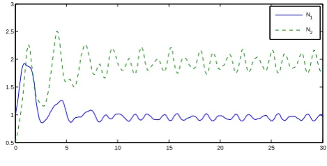
By a easy computation, it is not difficult to verify that(F3)
-(F5)in Theorem 3 and(S1)in Theorem 8 are satisfied. By Theorem 3 and Theorem 8, system (6.1) admits at least one positive almost periodic solution (see Figure 4.1), which is globally asymptotic stable.
title(’yslice:600m;zslice:150m’,’FontName’,’Times New Roman’,’FontSize’,22);
0 5 10 15 20 25 30 0.5
1 1.5 2 2.5 3
N1
N2
Fig. 1 State variablesN1 andN2 of Example 2
Remark 3. In Example 4, |sin√10t| is
√ 10π
10 -periodic function and |cos(√5t)| is
√ 5π
5 -periodic function. So sys-tem (6.1) is with incommensurable periods. Through all the coefficients of system (6.1) are periodic functions, the positive periodic solutions of system (6.1) could not possibly exist. However, by Theorem 3, the positive almost periodic solutions of system (6.1) exactly exist (see Figure 1).
Example 5. In system (6.1), let
K1(t) K2(t)
=
|sin√5t|+|cos√10t| |cos√10t|
,
H1(t) H2(t)
=
sin2(√2t) cos2(√2t)
,
α1(t) α2(t)
=
2|sin√5t|+ 2|cos√10t|
2|cos√10t|
,
β1(t) β2(t)
=
sin2(√2t) + 0.5 cos2(√2t) + 0.5
.
In Example 4, |sin√5t|+|cos√10t| is almost periodic function, which is not periodic function. Similar to the argument as that in Example 2, it is easy to obtain that system (6.1) admits at least one positive almost periodic solution.
Example 6. In system (6.1), let
K1(t) K2(t)
=
1.5 +|sint|
2.5 +|cost|
,
H1(t) H2(t)
=
0.5 + sin2t
0.5 + cos2t
,
α1(t) α2(t)
=
sin2t
cos2t
,
β1(t) β2(t)
=
sin2t
cos2t
.
By a easy computation, it is not difficult to verify that(F3)
-(F5) in Corollary 5 are satisfied. By Corollary 5, system (6.1) admits at least one positiveπ-periodic solution.
Remark 4. It is obvious that the results in papers [4,5,30]
couldn’t obtain the existence of positive (almost) periodic solutions for the models in Example 2 and Examples 4-5. Therefore, our works extend the results in papers [4,5,30].
ACKNOWLEDGEMENTS
This work is supported by the Scientific Research Fund of Yunnan Provincial Education Department (2014Y388) and the Research Program of Kunming University in China (XJL15010).
IAENG International Journal of Applied Mathematics, 48:2, IJAM_48_2_09
[image:8.595.313.548.63.182.2]REFERENCES
[1] D.H. Janzen, Coevolution of mutualism between ants and acacias in Central America, Evolution 20 (1966) 249-275.
[2] K.G. Porter, Enhancement of algal growth and productivity by grazing zooplankton, Science 192 (1976) 1332-1334.
[3] K. Gapalsamy, Stability and Oscillations in Delay Equations of Popu-lation Dynamics, Kluwer Academic Publishers, 1992.
[4] Y.K. Li, On a periodic mutualism model, ANZIAM J. 42 (2001) 569-580.
[5] Y.K. Li, G.T. Xu, Positive periodic solutions for an integrodifferential model of mutualism, Appl. Math. Lett. 14 (2001) 525-530.
[6] T.W. Zhang, Y.K. Li, Y. Ye, On the existence and stability of a unique almost periodic solution of Schoener’s competition model with pure-delays and impulsive effects, Communications in Nonlinear Science and Numerical Simulation 17 (2012) 1408-1422.
[7] T. W. Zhang, X. R. Gan, Existence and permanence of almost periodic solutions for Leslie-Gower predator-prey model with variable delays, Elect. J. Differ. Equa. 2013 (2013) 1-21.
[8] T. W. Zhang, X. R. Gan, Almost periodic solutions for a discrete fishing model with feedback control and time delays, Commun. Nonlinear Sci. Numer. Simulat..19 (2014) 150-163.
[9] Y.Q. Li, T.W. Zhang, Existence and multiplicity of positive almost periodic solutions for a non-autonomous SIR epidemic model, Bull. Malays. Math. Sci. Soc. 39 (2016) 359-379.
[10] Y.Q. Li, T.W. Zhang, Almost periodic dynamics in a nonautonomous bi-directional consumer-resource system with time delays, Comp. Appl. Math. 35 (2016) 559-577.
[11] T.W. Zhang, Multiplicity of positive almost periodic solutions in a delayed Hassell-Varley type predator-prey model with harvesting on prey, Math. Meth. Appl. Sci. 37 (2013) 686-697.
[12] T.W. Zhang, Almost periodic oscillations in a generalized Mackey-Glass model of respiratory dynamics with several delays, Int. J. Biomath. 7 (2014) 1-22.
[13] M. Fan, K. Wang, D.Q. Jiang, Existence and global attractivity of positive periodic solutions of periodicn-species Lotka-Volterra com-petition systems with several deviating arguments, Math. Biosci. 160 (1999) 47-61.
[14] Y.K. Li, Periodic solutions for delay Lotka-Volterra competition sys-tems, J. Math. Anal. Appl. 246 (2000) 230-244.
[15] Y. Chiba, T. Nose, M. Ito, A. Ito, Estimating the user’s state before exchanging utterances using intermediate acoustic features for spoken dialog systems, IAENG International Journal of Computer Science, vol. 43, no.1, pp1-9, 2016.
[16] W.L. Al-Yaseen, Z.A. Othman, M. Nazri, ”Real-time intrusion detec-tion system using multi-agent system,” IAENG Internadetec-tional Journal of Computer Science, vol. 43, no.1, pp80-90, 2016.
[17] Z. Chen, Y. Zhu, Y. Di, S. Feng, ”Optimized self-adaptive fault tolerance strategy in simulation system based on virtualization tech-nology,” IAENG International Journal of Computer Science, vol. 42, no.4, pp305-312, 2015.
[18] Z.Q. Zhang, X.W. Zheng, A periodic stage-structure mode, Appl. Math. Lett. 16 (2003) 1053-1061.
[19] H.F. Huo, W.T. Li, Positive periodic solutions of a class of delay differential system with feedback control, Appl. Math. Comput. 148 (2004) 35-46.
[20] F.D. Chen, Positive periodic solutions of neutral Lotka-Volterra system with feedback control, Appl. Math. Comput. 162 (2005) 1279-1302. [21] Z.Q. Zhang, L. Wang, Global attractivity of a positive periodic solution
for a nonautonomous stage structured population dynamics with time delay and diffusion, J. Math. Anal. Appl. 319 (2006) 17-33. [22] C.J. Zhao, On a periodic predator-prey system with time delays, J.
Math. Anal. Appl. 331 (2007) 978-985.
[23] K. Wang, Y.L. Zhu, Global attractivity of positive periodic solution for a Volterra model, Appl. Math. Comput. 203 (2) (2008) 493-501. [24] K. Wang, Existence and global asymptotic stability of positive periodic
solution for a predator-prey system with mutual interference, Nonlinear Anal.: RWA 10 (2009) 2774-2783.
[25] Y.L. Zhu, K. Wang, Existence and global attractivity of positive periodic solutions for a predator-prey model with modified Leslie-Gower Holling-type II schemes, J. Math. Anal. Appl. 384 (2011) 400-408.
[26] G.D. Zhang, Y. Shen, B.S. Chen, Positive periodic solutions in a non-selective harvesting predator-prey model with multiple delays, J. Math. Anal. Appl. 395 (2012) 298-306.
[27] A.M. Fink, Almost Periodic Differential Equations, Springer, Berlin, 1974.
[28] C.Y. He, Almost Periodic Differential Equations, Higher Education Publishing House, Beijing, 1992 (Chinese).
[29] R.E. Gaines, J.L. Mawhin, Coincidence Degree and Nonlinear Differ-ential Equations, Springer, Berlin, 1977.
[30] Y.K. Li, H.T. Zhang, Existence of periodic solutions for a periodic mutualism model on time scales, J. Math. Anal. Appl. 343 (2008) 818-825.
[31] Y. Xie, X.G. Li, Almost periodic solutions of single population model with hereditary effects, Appl. Math. Comput. 203 (2008) 690-697.