The Nonlinear HSS-like Iterative Method for
Absolute Value Equations
Mu-Zheng Zhu
†Member, IAENG,
and Ya-E Qi
‡Abstract—The Picard-HSS iterative method is proposed to solve the absolute value equation (AVE). To further improve its performance, a nonlinear HSS-like iterative method is pro-posed. Compared to that the Picard-HSS method is an inner-outer double-layer iterative scheme, the proposed nonlinear HSS-like iteration is only a monolayer iterative method and the iteration vector could be updated timely. Some numerical experiments are used to demonstrate that the nonlinear HSS-like method is feasible, robust and effective.
Index Terms—absolute value equation, nonlinear HSS-like iteration, fixed point iteration, positive definite.
I. INTRODUCTION
T
HE solution of the absolute value equation (AVE) with the following form is considered:Ax− |x|=b. (1)
Here,A∈Rn×n,x,b∈Rn and|x|denotes the component-wise absolute value of vectorx, i.e.,
|x|= (|x1|,|x2|, ...,|xn|)T.
The AVE (1) is a special case of the generalized absolute value equation (GAVE) of the type
Ax−B|x|=b, (2)
where A,B ∈Rm×n and x, b ∈Rm. The GAVE (2) was introduced in [1] and investigated in a more general context in [2]–[4]. Recently, these problems have been investigated in the literature [4]–[8].
The AVE (1) arises in linear programs, quadratic pro-grams, bimatrix games and other problems, which can all be reduced to a linear complementarity problem (LCP) [9]–[11], and the LCP is equivalent to the AVE (1). This implies that AVE is NP-hard in its general form [4], [6], [7]. Beside, if B=0, then the generalized AVE (2) reduces to the system of linear equationsAx=b, which have many applications in scientific computation[7],[12],[13].
The main research of the AVE includes two aspects: one is the theoretical analysis, which focuses on the theorem of alternatives, various equivalent reformulations, and the existence of solutions; see [1],[2],[5],[14]. And the other is how to solve the AVE. We mainly pay attention to the latter.
In the last decade, based on the fact that the LCP is equivalent to the AVE and the special structure of AVE,
Manuscript received January 11, 2018; This work was supported by the National Natural Science Foundation of China(11661033) and the Scientific Research Foundation for Doctor of Hexi University.
†Mu-Zheng Zhu is with the School of Mathematics and Statistics, Hexi University, Zhangye, 734000 P. R. China; E-mail: [email protected]. ‡Ya-E Qi is corresponding author, with the School of Chemistry and Chemical Engineering, Hexi University, Zhangye 734000 P.R. China; E-mail: [email protected].
a large variety of methods for solving AVE (1) can be found in the literature; See [3], [7], [8], [15]. The finite succession of linear programs (SLP) is established in[6], [15], which arise from a reformulation of the AVE as the minimization of a piecewise-linear concave function on a polyhedral set and solving the latter by successive lin-earization. Mangasarian[16]and Caccetta[14]present the semi-smooth Newton method and the smoothing Newton method to solve the AVE, respectively. In 2015, Haghani [17] propose an improved Newton method with two-step form, called Traub’s method, whose effectiveness is better than that of Mangasarian in [16]. To utilize the semi-smooth property, the generalized Newton method[18], the modified generalized Newton method [19], the improved generalized Newton method [20] and the inexact semi-smooth Newton algorithm[21]are further put forward for solving the AVE. These methods are all globally convergent under certain conditions.
Recently, the Picard-HSS iterative method is proposed to solve AVE by Salkuyeh in [22], which is originally designed to solve weakly nonlinear systems [23] and its generalizations are also paid attention[24],[25]. The suf-ficient conditions to guarantee the convergence and some numerical experiments are given to show the effectiveness of the method. However, the numbers of the inner HSS iteration steps are often problem-dependent and difficult to be determined in actual computations. Moreover, the iteration vector can not be updated timely. In this paper, we present the nonlinear HSS-like iterative method to overcome the defect of the mentioned above method in [22].
The rest of this paper is organized as follows. In Sec-tion II, the HSS and Picard-HSS iteraSec-tion methods are reviewed. In Section III, the nonlinear HSS-like iterative method for solving AVE (1) is described. Numerical ex-periments are presented in Section IV, to further shown the feasibility and effectiveness of the nonlinear HSS-like method. Finally, some conclusions are draw in Section V.
II. THEHSSANDPICARD-HSSITERATION METHODS
I
N this section, the HSS iterative method for solving the non-Hermitian linear systems and the Picard-HSS iterative method for solving the AVE (1) are reviewed.Let A ∈ Rn×n be a non-Hermitian positive definite matrix, B∈Rn×n be a zero matrix, the GAVE (2) reduced to the non-Hermitian system of linear equations
Ax=b. (3)
Because any square matrixApossesses a Hermitian and skew-Hermitian splitting (HSS)
A=H+S, H=1
2(A+A
H) and S=1
2(A−A
H), (4)
IAENG International Journal of Applied Mathematics, 48:3, IJAM_48_3_10
the following HSS iterative method is first introduced by Bai, Golub and Ng in [26] for solving the non-Hermitian positive definite system of linear equations (3).
Algorithm 1. (The HSS iterative method.)
Given an initial guess x(0) ∈ Rn, compute x(k) for k =
0, 1, 2, ... using the following iterative scheme until
{x(k)}∞
k=0 converges,
¨
(αI+H)x(k+12)= (αI−S)x(k)+b,
(αI+S)x(k+1)= (αI−H)x(k+1 2)+b,
whereαis a positive constant and I is the identity matrix.
When the Hermitian part H=12(A+AH) of the matrix A is positive definite, Bai et al. proved that the spectral radius of the HSS iteration matrix is less than 1 for any positive parameters α, i.e., the HSS iterative method is unconditionally convergent; see [26].
For the convenience of the subsequent discussion, the AVE (1) can be rewritten as its equivalent form:
Ax=f(x), f(x) =|x|+b.
Recalling that the linear termAxand the nonlinear term
f(x) =|x|+b are well separated and the Picard iterative method is a fixed-point iteration, the Picard iteration
Ax(k+1)=f(x(k)), k=0, 1, ....,
can be used to solve the AVE (1). When the matrix
A∈Rn×n is large sparse and positive definite, the next iteration x(k+1) may be inexactly computed by HSS
itera-tion. This naturally lead to the following iterative method proposed in[22] for solving the AVE (1).
Algorithm 2. (The Picard-HSS iterative method)
Let A∈Rn×n be a sparse and positive definite matrix, H=
1 2(A+A
H) and S= 1 2(A−A
H) be its Hermitian and
skew-Hermitian parts respectively. Given an initial guess x(0)∈
Rn and a sequence {`k}∞k=0 of positive integers, compute
x(k+1) for k=0, 1, 2, . . .using the following iterative scheme
until {x(k)}satisfies the stopping criterion:
(1) Set x(k,0):=x(k);
(2) For ` = 0, 1, . . . ,`k −1, solve the following linear systems to obtain x(k,`+1):
¨
(αI+H)x(k,`+1
2)= (αI−S)x(k,`)+|x(k)|+b,
(αI+S)x(k,`+1)= (αI−H)x(k,`+1
2)+|x(k)|+b,
where α is a given positive constant and I is the identity matrix;
(3) Set x(k+1):=x(k,`k).
The advantage of the Picard-HSS iterative method is obvious. Firstly, the two linear sub-systems in all inner HSS iterations have the same shifted Hermitian coefficient matrix αI +H and shifted skew-Hermitian coefficient matrix αI +S, which are constant with respect to the iteration indexk. Secondly, as the coefficient matrixαI+H
andαI+S are Hermitian and skew-Hermitian respectively, the first sub-system can be solved exactly by making use of the Cholesky factorization and the second one by the LU factorization. The lastly, these two sub-systems can be solve approximately by the conjugate gradient method and a Krylov subspace method like GMRES, respectively; see [22],[23].
III. THE NONLINEARHSS-LIKE ITERATIVE METHOD
I
N the Picard-HSS iteration, the numbers `k, k =0, 1, 2, ... of the inner HSS iteration steps are often problem-dependent and difficult to be determined in actual computations [23]. Moreover, the iteration vector can not be updated timely. Thus, to avoid these defect and still preserve the advantages of the Picard-HSS iterative method, based on the HSS (4) and the nonlinear fixed-point equations
(αI+H)x= (αI−S)x+|x|+b,
and
(αI+S)x= (αI−H)x+|x|+b,
the following nonlinear HSS-like iterative method is pro-posed to solve the AVE (1).
Algorithm 3. (The nonlinear HSS-like iterative method.) Let A∈Rn×n be a sparse and positive definite matrix, H=
1 2(A+A
H) and S= 1 2(A−A
H) be its Hermitian and
skew-Hermitian parts, respectively. Given an initial guess x(0)∈
Rn, compute x(k+1) for k =0, 1, 2, . . . using the following
iterative scheme until{x(k)}satisfies the stopping criterion:
¨
(αI+H)x(k+1
2)= (αI−S)x(k)+|x(k)|+b,
(αI+S)x(k+1)= (αI−H)x(k+1 2)+|x(k+
1 2)|+b,
whereα is a given positive constant and I is the identity matrix.
It is obvious that both x and |x| in the second step are updated in the nonlinear HSS-like iteration, but only
x is updated in the Picard-HSS iteration. Furthermore, the nonlinear HSS-like iteration is a monolayer iterative scheme, and the Picard-HSS is an inner-outer double-layer iterative scheme.
To obtain a one-step form of the nonlinear HSS-like iteration, the following symbols are introduced
U(x) = (αI+H)−1((αI−S)x+|x|+b),
V(x) = (αI+S)−1((αI−H)x+|x|+b),
and
ψ(x):=V◦U(x) =V(U(x)).
Then the nonlinear HSS-like iterative scheme can be equivalently expressed as
x(k+1)=ψ(x(k)).
The Ostrowski theorem, i.e., Theorem 10.1.3 in [27], gives a local convergence theory about a one-step s-tationary nonlinear iteration. Based on this, Bai et al. established the local convergence theory for the nonlinear HSS-like iterative method in [23]. However, this conver-gence theory has a strict requirement that f(x) =|x|+b
must be F-differentiable at a point x∗ ∈ D such that Ax∗− |x∗|=b. Obviously, the absolute value function |x|
is non-differentiable. Thus, the convergence analysis of the nonlinear HSS-like iterative method for solving weakly nonlinear linear systems is unsuitable for solving AVE, and need further discuss.
At the end of this section, we remark that the nonlinear HSS-like iterative method can be alternatively reformulat-ed into residual-updating form as follows.
IAENG International Journal of Applied Mathematics, 48:3, IJAM_48_3_10
Algorithm 4. (The residual-updating variant of the nonlin-ear HSS-like method) Given an initial guess x(0)∈D⊂Rn, compute x(k+1)for k=0, 1, 2, . . .using the following iterative
procedure until{x(k)}satisfies the stopping criterion:
(1) Set r(k):=|x(k)|+b−Ax(k),
(2) Solve (αI+H)v=r(k),
(3) Set x(k+1
2)=x(k)+v , r(k):=|x(k+ 1
2)|+b−Ax(k+ 1 2),
(4) Solve (αI+S)v=r(k),
(5) Set x(k+1)=x(k+1 2)+v ,
where α is a given positive constant and I is the identity matrix.
IV. NUMERICAL EXPERIMENTS
I
N this section, the numerical properties of the Picard, Picard-HSS and nonlinear HSS-like methods are ex-amined and compared experimentally by a suit of test problems.All the tests are performed in MATLAB R2013a on Intel(R) Core(TM) i5-3470 CPU 3.20 GHz and 8.00 GB of RAM, with machine precision 10−16, and terminated when
the current residual satisfies
kAx(k)− |x(k)| −bk2
kbk2 ≤
10−5,
where x(k) is the computed solution by each of the
methods at iteration k, and a maximum number of the iterations 500 is used.
In addition, the stopping criterion for the inner itera-tions of the Picard-HSS method is set to be
kb(k)−A s(k,`k)k2
kb(k)k2 ≤ηk,
where b(k)=|x(k)|+b−Ax(k), s(k,`k)=x(k,`k)−x(k,`k−1), `k
is the number of the inner iteration steps and ηk is the
prescribed tolerance for controlling the accuracy of the inner iterations at the k-th outer iteration. Ifηk is fixed
for all k, then it is simply denoted by η. Here, we take η=0.1.
The first subsystem with the Hermitian positive definite coefficient matrix(αI+H)in (3) is solved by the Cholesky factorization, and the second subsystem with the skew-Hermitian coefficient matrix (αI+S) in (3) is solved by the LU factorization.
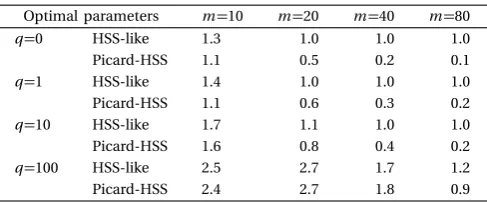
The optimal parameters employed in the Picard-HSS and nonlinear HSS-like iteration methods have been ob-tained experimentally. In fact, the experimentally found optimal parameters are the ones resulting in the least numbers of iterations and CPU times [22]. As mentioned in [23] the computation of the optimal parameter is often problem-dependent and generally difficult to be determined.
We consider the two-dimensional convection-diffusion equation
(
−(ux x+uy y) +q(ux+uy) +p u=f(x,y), (x,y)∈Ω, u(x,y) =0, (x,y)∈∂Ω,
whereΩ = (0, 1)×(0, 1),∂Ωis its boundary,q is a positive constant used to measure the magnitude of the diffusive term and p is a real number.
Leth=1/(m+1) andRe= (q h)/2 denote the equidis-tant step size and the mesh Reynolds number, respectively. We use the five-point finite difference scheme to the diffusive term and the central difference scheme to the convective term. Then we get a system of linear equations
Ax=d, whereA is a matrix of ordern=m2 of the form
A=Tx⊗Im+Im⊗Ty+p In, (5)
with
Tx=tridiag(t2,t1,t3)m×m andTy=tridiag(t2, 0,t3)m×m,
wheret1=4, t2=−1−Re, t3=−1+Re,Im andIn are the
identity matrices of orderm andn respectively,⊗means the Kronecker product.
In our numerical experiments, the matrix A in AVE (1) is defined by (5) with different values of q(q =
0, 1, 10, 100 and 1000) and p(p =0 and 0.5). It is easy to find that the matrixAis in general non-symmetric positive definite for any nonnegative number q [22]. The zero vector is used as the initial guess, and the right-hand side vectorb of AVE (1) is taken in such a way that the vector
x= (x1,x2, . . . ,xn)T withxk= (−1)k i (k=1, 2, . . . ,n) is the
[image:3.595.305.549.375.476.2]exact solution, where i denotes the imaginary unit.
TABLE I: The optimal parameters valuesα(p=0).
Optimal parameters m=10 m=20 m=40 m=80
q=0 HSS-like 1.3 1.0 1.0 1.0
Picard-HSS 1.1 0.5 0.2 0.1
q=1 HSS-like 1.4 1.0 1.0 1.0
Picard-HSS 1.1 0.6 0.3 0.2
q=10 HSS-like 1.7 1.1 1.0 1.0
Picard-HSS 1.6 0.8 0.4 0.2
q=100 HSS-like 2.5 2.7 1.7 1.2
Picard-HSS 2.4 2.7 1.8 0.9
TABLE II: The optimal parameters valuesα(p=0.5).
Optimal parameters m=10 m=20 m=40 m=80
q=0 HSS-like 2.4 2.2 2.1 2.0
Picard-HSS 2.2 2.0 1.8 1.8
q=1 HSS-like 2.4 2.2 2.1 2.0
Picard-HSS 2.3 2.0 1.8 1.8
q=10 HSS-like 2.6 2.3 2.2 2.1
Picard-HSS 2.4 2.3 2.0 1.9
q=100 HSS-like 3.4 2.9 2.3 2.3
Picard-HSS 3.5 3.0 2.3 2.1
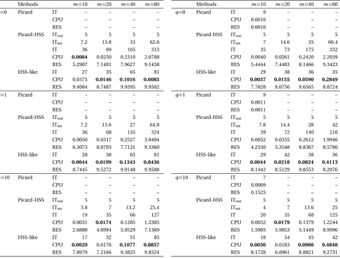
The numerical results of the Picard, Picard-HSS and nonlinear HSS-like iterations are list in Tables III and IV, and the experimentally optimal parameters used in the Picard-HSS and nonlinear HSS-like iterations are those given in Tables I and II. We give the elapsed CPU time in seconds for the convergence (denoted as CPU), the norm of absolute residual vectors (denoted as RES), and the number of outer, inner and total iteration steps (outer and inner iterations only for Picard-HSS) for the convergence (denoted as ITout, ITint and IT, respectively). The number
of outer iteration steps for Picard-HSS and the number of iteration steps for Picard and HSS-like iteration methods larger than 500 are simply listed by the symbol "–".
IAENG International Journal of Applied Mathematics, 48:3, IJAM_48_3_10
[image:3.595.303.551.518.618.2]From these two tables, we see that both the HSS-like and Picard-HSS methods can successfully produced approximate solution to the AVE for all of the problem-scalesn=m2 and the convective measurementsq, while
the Picard iteration converges only for some special cases. Here, it is necessary to mention that the shifted matrices αI+H andαI+S are usually more well-conditioned than the matrix A[22].
For the convergent cases, the number of iteration steps for the Picard and HSS-like methods and the number of inner iteration steps for the Picard-HSS method are increase rapidly with the increasing of problem-scale, while the number of outer iteration steps is fixed. The CPU time also increases rapidly with the increasing of the problem-scale for all iteration methods.
When the convective measurementsqbecome large, for all iterative method, both the number of iteration steps (except outer iteration for Picard-HSS) and the amount of CPU times decrease slightly.
Clearly, the iteration steps of the nonlinear HSS-like method are more robust than those of the Picard-HSS, and the iteration steps of the Picard method are more than 500 , then the nonlinear HSS-like method performs much better than the Picard-HSS in terms of iteration step; In terms of CPU time, the situation is almost the same, i.e., the nonlinear HSS-like iterative method is the
TABLE III: Numerical results for test problems with differ-ent values of m andq (p=0, RES(×10−6) ).
Methods m=10 m=20 m=40 m=80
q=0 Picard IT – – – –
CPU – – – –
RES – – – –
Picard-HSS ITout 5 5 5 5
ITint 7.2 13.8 33 62.6
IT 36 69 165 313
CPU 0.0084 0.0250 0.2310 2.0708 RES 5.2907 7.1401 7.9627 9.1458
HSS-like IT 27 35 65 81
CPU 0.0375 0.0146 0.1016 0.6085 RES 9.4084 8.7487 9.9395 9.9502
q=1 Picard IT – – – –
CPU – – – –
RES – – – –
Picard-HSS ITout 5 5 5 5
ITint 7.2 13.6 27 64.8
IT 36 68 135 324
CPU 0.0050 0.0317 0.2527 3.0404 RES 6.3073 8.0703 7.7121 9.3360
HSS-like IT 28 38 65 81
CPU 0.0044 0.0199 0.1343 0.8436 RES 8.7445 9.5272 9.9148 9.9588
q=10 Picard IT – – – –
CPU – – – –
RES – – – –
Picard-HSS ITout 5 5 5 5
ITint 3.8 7 13.2 25.4
IT 19 35 66 127
CPU 0.0031 0.0174 0.1285 1.2305 RES 2.6888 4.0994 5.9529 7.1369
HSS-like IT 17 32 51 85
CPU 0.0029 0.0176 0.1077 0.8857 RES 7.8979 7.2166 9.3825 9.8324
most time-efficient in the convergent cases. Therefore, the nonlinear HSS-like method are the winners for solving this test problem when the convective measurementsqis not large.
V. CONCLUSIONS
I
N this paper, the nonlinear HSS-like iterative method is proposed to solve the absolute value equation (AVE), which is based on two aspects: the first is the separable property of the linear term Ax and nonlinear term|x|+ b, and the second is the Hermitian and skew-Hermitian splitting of the involved matrix A. Compared to that the Picard-HSS iterative scheme is an inner-outer double-layer iterative scheme, the new nonlinear HSS-like iteration is a monolayer iterative method and the iteration vector could be updated timely. Numerical experiments have shown that the nonlinear HSS-like method is feasible, robust and efficient nonlinear solver.ACKNOWLEDGEMENTS
[image:4.595.57.547.415.786.2]The author would like to thank the anonymous referees for his/her careful reading of the manuscript and useful comments and improvements.
TABLE IV: Numerical results for test problems with differ-ent values ofm andq (p=0.5, RES(×10−6) ).
Methods m=10 m=20 m=40 m=80
q=0 Picard IT 9 – – –
CPU 0.0010 – – –
RES 0.0016 – – –
Picard-HSS ITout 5 5 5 5
ITint 7 14.6 35 66.4
IT 35 73 175 332
CPU 0.0040 0.0261 0.2420 2.2039 RES 5.4444 7.4483 8.1466 9.3423
HSS-like IT 29 38 36 35
CPU 0.0037 0.0155 0.0590 0.2849 RES 7.7828 8.0756 9.6565 8.8724
q=1 Picard IT 9 – – –
CPU 0.0011 – – –
RES 0.0011 – – –
Picard-HSS ITout 5 5 5 5
ITint 7.8 14.4 28 42
IT 39 72 140 210
CPU 0.0052 0.0335 0.2612 1.9946 RES 4.2330 5.3548 8.8367 8.5786
HSS-like IT 29 42 38 36
CPU 0.0044 0.0218 0.0824 0.4113 RES 8.1442 8.5129 9.8553 8.2976
q=10 Picard IT 7 – – –
CPU 0.0009 – – –
RES 0.1525 – – –
Picard-HSS ITout 5 5 5 5
ITint 4 7 13.6 25
IT 20 35 68 125
CPU 0.0032 0.0179 0.1379 1.2244 RES 1.5905 5.9853 5.1449 8.9996
HSS-like IT 18 34 45 42
CPU 0.0030 0.0183 0.0960 0.4848 RES 8.1728 6.0961 8.8821 9.2731
IAENG International Journal of Applied Mathematics, 48:3, IJAM_48_3_10
REFERENCES
[1] J. Rohn, “A theorem of the alternatives for the equationa x+b|x|=
b,”Linear Multilinear Algebra, vol. 52, no. 6, pp. 421–426, 2004.
[2] S.-L. Hu and Z.-H. Huang, “A note on absolute value equations,”
Optimization Letters, vol. 4, no. 3, pp. 417–424, 2010.
[3] O. L. Mangasarian, “Primal-dual bilinear programming solution of the absolute value equation,”Optimization Letters, vol. 6, no. 7, pp. 1527–1533, 2012.
[4] O. L. Mangasarian and R. R. Meyer, “Absolute value equations,”
Linear Algebra and its Applications, vol. 419, pp. 359–367, 2006.
[5] O. Prokopyev, “On equivalent reformulations for absolute value equations,”Computational Optimization and Applications, vol. 44, no. 3, pp. 363–372, 2009.
[6] O. L. Mangasarian, “Absolute value equation solution via concave minimization,”Optimization Letters, vol. 1, no. 1, pp. 3–8, 2007.
[7] M. A. Noor, J. Iqbal, K. I. Noor, and E. Al-Said, “On an iterative method for solving absolute value equations,”Optimization Letters, vol. 6, no. 7, pp. 1027–1033, 2012.
[8] J. Rohn, V. Hooshyarbakhsh, and R. Farhadsefat, “An iterative method for solving absolute value equations and sufficient con-ditions for unique solvability,”Optimization Letters, vol. 8, no. 1, pp. 35–44, 2014.
[9] R. W. Cottle, J.-S. Pang, and R. E. Stone,The linear complementarity problem, vol. 60, SIAM, 2009.
[10] V. Klement, T. Oberhuber, “Multigrid method for linear comple-mentarity problem and its implementation on GPU,”IAENG Inter-national Journal of Applied Mathematics, vol. 45, no. 3, pp. 193–197, 2015.
[11] O. L. Mangasarian, “Solution of symmetric linear complementarity problems by iterative methods,”Journal of Optimization Theory and Applications, vol. 22, no. 4, pp. 465–485, 1977.
[12] A.-J. Li, “A new preconditioned AOR iterative method and compar-ison theorems for linear systems”,IAENG International Journal of Applied Mathematics, vol. 42, no. 3, pp. 161–163 , 2012.
[13] J. B. Erway, R. F. Marcia, and J. Tyson. “Generalized diagonal pivoting methods for tridiagonal systems without interchanges.”
IAENG International Journal of Applied Mathematics, vol. 40, no. 4, pp. 269–275, 2010.
[14] L. Caccetta, B. Qu, and G.-L. Zhou, “A globally and quadratically convergent method for absolute value equations,”Computational Optimization and Applications, vol. 48, no. 1, pp. 45–58, 2011.
[15] O. L. Mangasarian, “Knapsack feasibility as an absolute value equation solvable by successive linear programming,”Optimization Letters, no. 3, pp. 161–170, 2009.
[16] O. L. Mangasarian, “A generalized Newton method for absolute value equations,”Optimization Letters, no. 3, pp. 101–108, 2009.
[17] F. K. Haghani, “On generalized Traub’s method for absolute value equations,”Journal of Optimization Theory and Applications, vol. 166, no. 2, pp. 619–625, 2015.
[18] C. Zhang, Q.-J. Wei, “Global and finite convergence of a generalized Newton method for absolute value equations,”Journal of Optimiza-tion Theory and ApplicaOptimiza-tions, vol. 143, no. 2, pp. 391–403, 2009.
[19] C.-X. Li,“A modified generalized Newton method for absolute value equations,”Journal of Optimization Theory and Applications, vol. 170, no. 3, pp. 1055–1059, 2016.
[20] J. Feng, S. Liu, “An improved generalized Newton method for absolute value equations,”SpringerPlus, vol. 5, 1042, 2016.
[21] J. B. Cruz, O. P. Ferreira, L. F. Prudente, “On the global convergence of the inexact semi-smooth Newton method for absolute value equation,”Computational Optimization and Applications, vol. 65, no. 1, pp. 93–108, 2016.
[22] D. K Salkuyeh, “The Picard-HSS iterative method for absolute value equations,”Optimization Letters, vol. 8, no. 8, pp. 2191–2202, 2014.
[23] Z.-Z. Bai and X. Yang, “On HSS-based iteration methods for weakly nonlinear systems,Applied Numerical Mathematics, vol. 59, no. 12, pp. 2923–2936, 2009.
[24] M.-Z. Zhu,“Modified iteration methods based on the asymmetric HSS for weakly nonlinear systems,Journal of Computational Anal-ysis and Applications, vol. 15, no. 1, pp. 188–195, 2013.
[25] Z.-N. Pu and M.-Z. Zhu, “A class of iteration methods based on the generalized preconditioned Hermitian and skew-Hermitian splitting for weakly nonlinear systems,”Journal of Computational and Applied Mathematics, vol. 250, no. 1, pp. 16–27, 2013.
[26] Z.-Z. Bai, G. H. Golub, and M. K. Ng, “ Hermitian and skew-Hermitian splitting methods for non-skew-Hermitian positive definite linear systems,”SIAM Journal on Matrix Analysis and Applications, vol. 24, no. 3, pp. 603–626, 2003.
[27] J. M. Ortega and W. C. Rheinboldt, “Iterative solution of nonlinear equations in several variables”, vol. 30, SIAM, 2000.
[28] L.-Q. Yong, “Particle swarm optimization for absolute value equa-tions,”Journal of Computer Information Systems, vol. 6, no. 7, pp. 2359–2366, 2010.