Explicit Error Estimate for the Nonconforming Crouzeix-Raviart Finite Element

Explicit Error Estimate for the Nonconforming

Crouzeix-Raviart Finite Element

Yongwei Yang

Abstract—In this paper, we study the explicit expressions of the constants in the error estimate of the nonconforming finite element method. We obtain an explicit relation between the consistency error estimate and the geometric characters of the triangle, which together with the interpolation error estimate implies the final finite element error estimate. Furthermore, such explicit a priori error estimate can be used as computable error bound, which is also consistent with the maximal angle condition for the optimal error estimate of the nonconforming finite element method.

Index Terms—Nonconforming finite element, Explicit error estimate, Maximal angle condition, Crouzeix-Raviart element.

I. INTRODUCTION

A

S a very effective numerical method of partial differ-ential equations, the finite element method (FEM) is widely applied to the engineering and scientific computation. Furthermore, it also has formed firm theoretical bases such as a priori and a posteriori error estimations, seeing, e.g. ([1], [2], [3]). Let u, uh denote the exact solution of the model

problem and the associated discrete solution, respectively. The convergence analysis of the finite element method is typical of the form

∥u−uh∥ ≤Chk|u|, (I.1)

wherehdenotes the maximal diameter of the triangulation,

∥·∥and|·|stand for some appropriate norm and semi-norm in certain function spaces, respectively.

The constantCin (I.1) is independent of element size, but may dependent on the sine of the minimal angle of the tri-angulation for the 2-D case, which is equivalent to the well-known non-degenerate assumption or regular assumption of finite element meshes, seeing, e.g. ([4]). In fact, the minimal angle condition for the finite elements can be relaxed, which results in the so-called anisotropic elements or degenerate elements found long time before in [5]. Since late 1980’s the anisotropic elements have been extensively studied, ref. ([6], [7]) and references therein.

As is known that there also appear various constants in the process to derive the final error estimates. It is good to evaluate or bound these constants explicitly for a quantitative error bound purpose. Actually, there are some works on estimation of the error constants for the finite elements, see, e.g., ([8], [9], [10]) for linear triangular finite elements and ([11], [12]) for bilinear quadrilateral finite elements. However, almost all of them are concentrated on the standard conforming finite element method, which only involves an explicit interpolation error estimate. For the nonconforming

Manuscript received June 17, 2019; revised September, 23, 2019. This work was supported in part by Higher Education Key Scientific Research Program Funded by Henan Province (No. 20A110011, 20B630002).

Y. Yang is with the School of Mathematics and Statistics, Anyang Normal University, Anyang, Henan, 455000 China, e-mail: [email protected]

finite element method, an explicit error estimate for the Crouzeix-Raviart element is given in [13] by its close relation to the mixed finite element method. Note that Kikuchi and Liu [14] have derived an explicit interpolation error bound for the Crouzeix-Raviart element, but it can not imply an explicit bound for the finite element error.

In this paper, we still study explicit error estimate for the nonconforming Crouzeix-Raviart element for the Poisson problem. The difference between our method and that in [13] is that we obtain the explicit error bounds for the Crouzeix-Raviart element by the standard nonconforming finite element method in stead of its close relation to the mixed finite element method. Therefore, our method is more suitable for general nonconforming case. In this process, the finite element error of the nonconforming element can be explicitly estimated by the sum of an interpolation error and a consistency error, seeing section II. The interpolation error has been obtained by Kikuchi and Liu, seeing section III . In section IV, the consistency error is considered based on some anisotropic results given by Apel et al. in [15]. In section V, the results in sections III and IV are applied to obtain the explicit error estimate for the Poisson problem. Furthermore, our explicit error estimate for the nonconforming element is consistent with the maximal angle condition. In section VI, we show by a numerical experiment that the experimentally determined constants are below the theoretical estimate given in section V. In the final section of the paper, we give some comments and extensions of the results.

II. DISCRETIZATION OF THE MODEL PROBLEM

In this paper, let Ω be a bounded convex polygonal domain, and the semi-norms in Sobolev space H2(Ω) be define by

|v|1,Ω= ( 2

∑

i=1

∥ ∂v ∂xi∥

2 0,Ω)

1 2_,

|v|2,Ω= ( 2

∑

i,j=1

∥ ∂2v ∂xi∂xj∥

2 0,Ω)

1 2_.

We consider the following Poisson problem: find u ∈ H01(Ω) such that{

−∆u=f, in Ω,

u= 0, on∂Ω, (II.1)

wheref ∈L2_(Ω).

It is known that for the convex domain with∂Ω∈C2_{, the}

above problem has a unique solutionu∈H2_(Ω)∩H1 0(Ω).

Furthermore, the following Miranda-Talente estimate holds, ref. ([16], [17]),

|u|2,Ω≤ ∥f∥0,Ω, (II.2)

which was extended to the general convex polygonal domain in [18].

IAENG International Journal of Applied Mathematics, 50:1, IJAM_50_1_16

The variational form of problem (II.1) is to find u ∈ H1

0(Ω)such that

(∇u,∇v) = (f, v), ∀v∈H01(Ω). (II.3)

Here, (·,·)Ω denotes the inner products of both L2_(Ω)

and L2_(Ω)2_{, where the subscript Ω is often omitted. The}

existence and uniqueness of variational solution uof (II.3) follows from Lax-Milgram lemma.

Let Th be a finite element triangulation of Ω. Based on

Th, we introduce the Crouzeix-Raviart finite element space Vh,

{

vh∈L2(Ω);vh|T ∈P1(T),

∫

l

[vh]ds= 0,∀l⊆∂T, ∀T ∈ Th

}

,

where[vh]is the jump of the function vh on the edge. And

for boundary edges, we identify [vh]withvh.

We note that Vh*H01(Ω), which means that the method

is nonconforming. Thus∇vhis not defined on inter-element

boundaries and we define the finite solutionuh by using the

weaker inner product

(u, v)h,∑ T

(u, v)T,

that is to finduh∈Vh such that

(∇uh,∇vh)h= (f, vh),∀vh∈Vh.

Similar to the proof of the second Strang’s lemma [1], the finite element erroru−uh can be explicitly estimated in the

norm∥ · ∥h, that is,

∥u−uh∥h≤ inf vh∈Vh

∥u−vh∥h

+ sup vh∈Vh

|(∇u,∇vh)h−(f, vh)|

∥vh∥h

,

(II.4)

where∥vh∥h = (

∑

T

|vh|21,T)

1

2. The two terms are called an

approximation error and a consistency error, respectively. The approximation error is estimated by using vh = Ihv

with a suitably defined interpolation operator Ih, seeing the

next section. A general discussion of the consistency error is given in section IV .

III. APPROXIMATION ERROR ESTIMATE

In this section, we mainly present the results given by Kikuchi and Liu, ref. [14]. To this end, let hT, aT andθT

be positive constants such that

hT >0, 0< aT ≤1, (π

3 ≤) cos

−1aT

2 ≤θT < π.

(III.1)

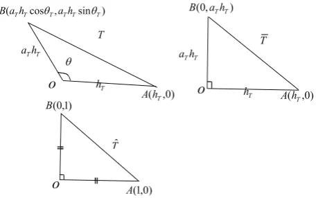
Then we define the triangle TaT,θT,hT by △OAB with three vertices O(0,0), A(hT,0) and B(aThTcosθT, aThTsinθT). From (III.1),∠AOB=θT is

the maximum interior angle and ABthe edge of maximum length, i.e., |AB| ≥ hT ≥ aThT, so that hT = |OA|

denotes the medium edge length, although the notation

hT is often used as the largest edge length. Since we can

configure any triangle T as TaT,θT,hT by an appropriate

congruent transformation in R2, without loss of generality we suppose that TaT,θT,hT is a general triangle T with the

edges l1 = OA, l2 = OB and l3 = AB. Then l2 is the

minimal edge and l1, l3 are two long edges. We will use

abbreviated notations T = TaT,θT,hT,T¯ = TaT,π₂,hT and

ˆ T =T1,π

2,1, seeing Fig. 1.

!"# $ %&! '"! "!

# #'($"!

$

!

( $ '! % !

"

$

!

( $ '! % !

"

) $ ( '

#

*

$

( $ ) '

[image:2.595.317.547.73.216.2]

%

Fig. 1. Notations for triangles:T =Ta_T,θT,hT,T¯ =TaT,π2,hT and

ˆ

T=T1,π 2,1

We define the following closed linear spaces for functions overT:

V_T0=

{

v∈H1(T);

∫

T

vdx= 0

}

, (III.2)

V_T1=

{

v∈H1(T);

∫

l1

vds= 0

}

, (III.3)

VT2=

{

v∈H1(T);

∫

l3

vds= 0

}

. (III.4)

To give the interpolation error estimate, we introduce the positive constants defined by

Ci(aT, θT, hT) = sup v∈Vi T

∥v∥0,T

|v|1,T

, i= 0,1,2. (III.5)

The existence of these constants follows from the standard compactness arguments. For convenience, we will use the abbreviated notationsCi(aT, hT) =Ci(aT,π₂, hT)andCi= Ci(1,π₂,1)for i= 0,1,2. We present the estimates of them as follows, ref. ([14], Theorems 1–4).

Lemma 3.1:

Ci(aT, θT, hT)≤Ci(aT, hT)(1 +|cosθT|)

1 2

≤Ci(1 +|cosθT|)

1 2_hT,

(III.6)

wherei= 0,1,2,

C0≤ 1 π, C1=C2, 0.49282≤C1≤0.49293.

(III.7)

The Crouzeix-Raviart interpolation Ih : H1(Ω) → Vh is

defined by_∫

l

Ihuds=

∫

l

uds,∀l⊂∂T, ∀T ∈ Th. (III.8)

We present the local error estimate for the interpolation Ih

which is given in [14].

Lemma 3.2: For anyv∈H2_{(T), we have}

v−Ihv_1,T ≤C0

(

1 +|cosθT|

)1 2_h

T|v|2,T. (III.9)

Therefore, according to Lemma 3.2 and (II.2) we set

vh = Ihu in the first term of (II.4), and then we get the

IAENG International Journal of Applied Mathematics, 50:1, IJAM_50_1_16

approximation error estimate

inf vh∈Vh

∥u−vh∥h≤ ∥u−Ihu∥h

= (∑ T

|u−Ihu|21,T)

1 2

≤√2C0h|u|2,Ω

≤√2C0h∥f∥0,Ω,

(III.10)

whereh= max T hT.

IV. CONSISTENCY ERROR ESTIMATE

A. Simple triangulation T¯h={T¯}

In this subsection, we discuss the explicit estimate of the consistency error over the simple triangulationT¯h. Firstly we

introduce a sharp trace theorem onTˆ.

Lemma 4.1: ∀v∈H1_{( ˆT), ∀ε >0, we have}

∥v∥2_0,ˆl

i ≤2(1 +

1 ε2)∥v∥

2 0,Tˆ+ε

2_|v|2

1,Tˆ, i= 1,2, (IV.1)

∥v∥2_0,ˆl

3 ≤2 √

2(1 + 2 ε2)∥v∥

2 0,Tˆ+ 2

√

2ε2|v|2_1,Tˆ. (IV.2)

Proof: The proof for (IV.1) can be found in [13]. Therefore we only need to give the proof of (IV.2).

By density, we assume that v ∈ C∞( ˆT). Let Kˆ be the unit square domain containingTˆ, i.e.,

ˆ

K={(x, y); 0≤x, y≤1}.

Then we can extendv toKˆ by reflection with respect to the line x+y= 1as following:

˜ v=

{

v(x, y), (x, y)∈T ,ˆ

v(1−y,1−x), (x, y)∈K/ˆ T .ˆ (IV.3)

Due to the symmetry ofv˜, we have

∥v˜∥2_0,Kˆ = 2∥v∥2_0,Tˆ,

∥∂v˜ ∂x∥

2

0,Kˆ =|v| 2 1,Tˆ,

∥∂˜v ∂y∥

2

0,Kˆ =|v| 2 1,Tˆ.

(IV.4)

Here we only prove the second equation in (IV.4), i.e.,

∥∂˜v ∂x∥

2 0,Kˆ =∥

∂˜v ∂x∥

2 0,Tˆ+∥

∂˜v ∂x∥

2 0,K/ˆ Tˆ =∥∂v

∂x∥ 2 0,Tˆ+

∫ 1 0

dx

∫ 1 1−x

(∂v(1−y,1−x)

∂x )

2_dy

=∥∂v ∂x∥

2 0,Tˆ+

∫ 1 0

dz

∫ 1−z 0

(∂v(t, z) ∂z )

2_dt

=|v|2_1,Tˆ.

The third one can be proved similarly and the first one is obvious. Consider the functionw∈C∞( ˆK), then

w2(ξ, η) =w2(x, y) + 2

∫ ξ x

w(t, η)∂w(t, η) ∂t dt

+ 2

∫ η y

w(x, z)∂w(x, z) ∂z dz

≤w2(x, y) + 2|

∫ ξ x

w(t, η)∂w(t, η) ∂t dt|

+ 2|

∫ η y

w(x, z)∂w(x, z) ∂z dz|.

(IV.5)

Integrating both sides of (IV.5) on ˆl3 and Kˆ, by simple

calculations we get_∫

ˆ l3

w2dˆs≤√2∥w∥2 0,Kˆ + 2

√

2∥w∥_0,Kˆ∥ ∂w ∂x∥0,Kˆ + 2√2∥w∥_0,Kˆ∥

∂w ∂y∥0,Kˆ ≤√2(1 + 2

ε2)∥w∥ 2 0,Kˆ +

√

2ε2|w|2_1,Kˆ.

(IV.6)

SinceC∞( ˆK)is dense inH1( ˆK), according to (IV.3–IV.4) and (IV.6) we obtain_∫

ˆ l3

v2dˆs=

∫

ˆ l3

˜ v2dˆs

≤√2(1 + 2 ε2)∥v˜∥

2 0,Kˆ +

√

2ε2|v˜|2_1,Tˆ

≤2√2(1 + 2 ε2)∥v∥

2 0,Tˆ+ 2

√

2ε2|v|2_1,Tˆ,

which is (IV.2).

LetP_T¯ :L1( ¯T)→P0( ¯T)andPl :L1(l)→P0(l) be the

averaging operator on the triangle T¯ and the edge l which preserve polynomials of degree zero, respectively. For the convenience of the subsequent discussion, we present the following estimates.

Lemma 4.2: For any v ∈ H1_{( ¯T) and v}

h ∈ P1( ¯T), we

have

∫_l

i

(v−P_T¯v)(vh−Plivh)ds

≤

√

(C2 0+

√

2C0)(C2 1+

√

2C1)

· |li|

|_T¯_|

( ∑

j=1,2

|lj|2∥ ∂v ∂xj∥

2 0,T¯

)1 2( ∑

j=1,2

|lj|2∥ ∂vh ∂xj∥

2 0,T¯

)1 2

,

i= 1,2,

(IV.7)

∫_l

3

(v−PT¯v)(vh−Pl3vh)ds

≤√(C2 0+

√

2C0)(

√

2C2 1+ 4C1

)

·|l3|

|_T¯_|

( ∑

j=1,2

|lj|2∥ ∂v ∂xj

∥2 0,T¯

)1 2( ∑

j=1,2

|lj|2∥ ∂vh ∂xj

∥2 0,T¯

)1 2

.

(IV.8)

Proof:By using transformation to the reference edgeˆli

and the Cauchy-Schwarz inequality, we obtain_∫

li

(v−PT¯v)(vh−Plivh)ds

=|li|

∫

ˆli

(ˆv−PTˆˆv)(ˆvh−Pˆ_livˆh)

≤ |li|

vˆ−P_Tˆvˆ

0,ˆli

vˆh−Pˆ_livˆh

0,ˆli .

(IV.9)

Fori= 1,2, combining (III.6) and (IV.1), we have

∥vˆ−P_Tˆvˆ∥2_0,ˆli ≤2(1 +

1

ε2)ˆv−PTˆˆv 2 0,Tˆ+ε

2_|ˆv|2 1,Tˆ

≤(2C₀2+2C 2 0 ε2 +ε

2_)|ˆv|2 1,Tˆ ε2₌√_2C

0

===== (2C02+ 2

√

2C0)|vˆ|2_1,Tˆ.

(IV.10) Since the transformation fromTˆ toT¯ leads to

(∂vˆ ∂xˆ1

)2+ ( ∂vˆ ∂xˆ2

)2=|l1|2( ∂v ∂x1

)2+|l2|2( ∂v ∂x2

)2. (IV.11)

IAENG International Journal of Applied Mathematics, 50:1, IJAM_50_1_16

Then (IV.10-IV.11) imply that

∥ˆv−P_Tˆˆv∥2_0,ˆ_l

i ≤

(C02+

√

2C0)

|_T¯_|

·

(

|l1|2∥ ∂v ∂x1

∥2

0,T¯+|l2|2∥ ∂v ∂x2

∥2 0,T¯

)

,

i= 1,2.

(IV.12) Similarly we also have

ˆvh−Pˆliˆvh

2

0,ˆli

≤ (C12+

√

2C1)

|_T¯_|

·

(

|l1|2∥ ∂vh ∂x1∥

2

0,T¯+|l2|2∥ ∂vh ∂x2∥

2 0,T¯

)

,

i= 1,2.

(IV.13) Combining (IV.9) and (IV.12–IV.13), we obtain (IV.7). For

i= 3, combining (III.5) and (IV.2), we proceeding along the same lines above and also obtain (IV.8).

Suppose w=∇u. In the sense of (II.4) it is our aim to derive an explicit estimate for

sup vh∈Vh

|(w,∇vh)h−(f, vh)|

∥vh∥h

. (IV.14)

To this end, we introduce an auxiliary finite element space

˜ Vh,

{

˜

vh∈L2(Ω); ˜vh|_T¯∈span{1, x2},

∫

li

[˜vh]ds= 0, i= 1,3, ∀T¯∈T¯h

}

,

which is sufficiently close toVh, ref. [15].

For any fixed∫ vh∈Vh, we definev˜h∈V˜h such that li

˜ vhds=

∫

li

vhds, i= 1,3, ∀T¯∈T¯h. (IV.15)

Both ∂vh

∂x2 and

∂˜vh

∂x2 are constants. Even better on

¯ T, we have

∂vh ∂x2

= ∂˜vh ∂x2

, (IV.16)

which is given in [15].

Combining (III.5–III.6) and (IV.15–IV.16) we have the following estimate

∥vh−v˜h∥0,T¯≤C1hT∥ ∂vh ∂x1

∥0,T¯. (IV.17)

We are now prepared to prove an explicit estimate for the consistency error over T¯h.

Lemma 4.3: For the simple triangulationT¯handw=∇u,

we have

sup vh∈Vh

|(w,∇vh)h−(f, vh)|

∥vh∥h

≤

[

C1+ 2

√

2

√

C2 0+

√

2C0

·(√C2 1+

√

2C1+

√_√

2C2 1+ 4C1

)]

h∥f∥0,Ω.

(IV.18)

Proof:Sincew=∇u, that is,−∇w=f, we introduce

˜

vhas above by using (IV.16) and Green’s formula as follows, (w,∇vh)h−(f, vh)

=∑ ¯ T

∫

¯ T

(

w1 ∂vh ∂x1

+w2 ∂˜vh ∂x2 −

f vh

)

dx

=−∑ ¯ T

∫

¯ T

(∂w1 ∂x1

vh+ ∂w2 ∂x2 ˜ vh+f vh

)

dx

+∑ ¯ T

∫

∂T¯

w1vhn1ds+

∑

¯ T

∫

∂T¯

w2˜vhn2ds

=∑ ¯ T

∫

¯ T

∂w2 ∂x2

(vh−˜vh)dx+

∑

¯ T

∫

∂T¯

w1vhn1ds

+∑ ¯ T

∫

∂T¯

w2˜vhn2ds.

(IV.19)

Combining the Cauchy-Schwarz inequality and (IV.17), we obtain the estimate of the first term of (IV.19)

∑

¯ T

∫

¯ T

∂w2 ∂x2

(vh−v˜h)dx

≤∑

¯ T

∂w2 ∂x2

0,T¯v−˜vh0,T¯

≤C1h

∑

¯ T

∂w2 ∂x2

0,T¯ ∂vh ∂x1

0,T¯

≤C1h|w2|1,Ω∥vh∥h.

(IV.20)

Consider the second term of (IV.19). Since

∑

¯ T

∑

l∈∂T¯\∂Ω

∫

l

w1n1ds= 0,

Plvh= 1

|l|

∫

l

vhds= 0, ∀l⊂∂Ω,

(IV.21)

we reformulate the second term by

∑

¯ T

∫

∂T¯

w1vhn1ds

=∑ ¯ T

∑

l_⊂∂T¯

∫

l

w1(vh−Plvh)n1ds.

(IV.22)

Furthermore, since∫_l(vh−Plvh)ds= 0for alll, we continue

with_∑

¯ T

∫

∂T¯

w1vhn1ds

=∑ ¯ T

∑

l⊂∂T¯

∫

l

(w1−PT¯w1)(vh−Plvh)n1ds.

(IV.23)

Since the outward unit normal toli⊂∂T¯ is

n=

        

(0,−1), i= 1, (−1,0), i= 2,

( aT

√

1 +a2 T

,√ 1 1 +a2

T

)

, i= 3,

(IV.24)

IAENG International Journal of Applied Mathematics, 50:1, IJAM_50_1_16

according to (IV.23) and Lemma 4.2, we obtain

∑

¯ T

∫

∂T¯

w1vhn1ds

≤∑

¯ T

∑

l_⊂∂T¯

n1

∫

l

(w1−P_T¯w1)(vh−Plvh)ds

≤∑

¯ T

[√

(C2 0+

√

2C0)(C2 1+

√

2C1)·|l2|

|_T¯_|h 2

Tw1_1,T¯vh_1,T¯ +√aT

1 +a2 T

·√(C2 0+

√

2C0)(√2C2 1+ 4C1)

·|l3|

|_T¯_|h 2

Tw1_1,T¯vh_1,T¯

] = 2 √ C2 0+ √

2C0

∑ ¯ T (√ C2 1+ √

2C1

+

√_√

2C2 1 + 4C1

)

hTw1_1,T¯vh1,T¯

≤2

√

C2 0+

√

2C0

(√

C2 1+

√

2C1

+

√_√

2C2 1 + 4C1

)

hw1_1,Ωvh_h.

(IV.25)

The third term of (IV.19) can also be explicitly estimated in the same way. We note only two new points. The first is thatPliv˜h= 0is in general only satisfied for the long edges l1, l3 ∈ ∂Ω, compare with the second term of (IV.21). For

the short edges l2∈∂Ω, we have to usen2 = 0. Secondly,

since ∂˜vh

∂x1 = 0 the term |l1|

2_∥∂v˜h

∂x1∥

2

0,T¯ vanishes. Hence the

estimate reads_∑

¯ T

∫

∂T¯

w2˜vhn2ds

≤∑

¯ T

∑

l_⊂T¯

n2

∫

l

(w2−PT¯w2)(˜vh−Pl˜vh)ds

≤∑

¯ T

[√

(C2 0+

√

2C0)(C2 1+

√

2C1)

·|l1|

|_T¯_|aThT2w2_1,T¯ ∂v˜h ∂x2

0,T¯

+

√

(C2 0+

√

2C0)(√2C2 1+ 4C1)

√

1 +a2 T

·|l3|

|_T¯_|aThT2w2_1,T¯ ∂v˜h ∂x2

0,T¯

] = 2 √ C2 0+ √

2C0

∑ ¯ T (√ C2 1+ √

2C1

+

√_√

2C2 1+ 4C1

)

hTw2_1,T¯ ∂vh ∂x2

0,T¯

≤2

√

C2 0+

√

2C0

(√

C2 1+

√

2C1

+

√_√

2C2 1+ 4C1

)

hw2_1,Ωvh_h,

(IV.26)

where we have also used (IV.16).

Combining (IV.19–IV.20), (IV.25–IV-A) and H¨older in-equality, we obtain

(w,∇vh)−(f, vh)

≤C1hw2_1,Ωvh_h+ 2

√

C2 0+

√

2C0

(√

C2 1+

√

2C1

+

√_√

2C₁2+ 4C1

)

h(w1_1,Ω+w2_1,Ω)vh_h

≤C1hw2_1,Ωvh_h+ 2

√

C2 0+

√

2C0

(√

C2 1+

√

2C1

+

√_√

2C2 1+ 4C1

)

hw1_1,Ωvh_h

≤

[

C1+ 2

√ 2 √ C2 0+ √

2C0

(√

C2 1+

√

2C1

+

√_√

2C2 1 + 4C1

)]

hw_1,Ωvh_h,

which together with (II.2) can imply (IV.18).

B. General triangulationTh={T}

In this subsection, we explicitly give the consistency error overTh based on that over T¯h.

Lemma 4.4: For the general triangulation Th and w =

∇u, putθ= max

T θT, we have sup

vh∈Vh

|(w,∇vh)h−(f, vh)|

∥vh∥h ≤

(√

2C1

√

sinθ+ 4

√

C2 0+

√

2C0

√

sinθ ·(√C2

1+

√

2C1+

√_√

2C2 1+ 4C1

))

h∥f∥0,Ω.

(IV.27)

Proof: Suppose F¯ is the transformation from T¯ to T

and₍¯v=v◦F¯, then we have

w,∇vh

)

h−

(

f, vh

) =∑ T ∫ T ( w1 ∂vh ∂x1

+w2 ∂vh ∂x2

−f vh

)

dx

=∑ T

sinθT

∫ ¯ T [ ¯ w1

∂¯vh ∂x¯1

+ ¯w2

(

−cosθT sinθT

∂v¯h ∂x¯1

+ 1 sinθT

∂¯vh ∂x¯2

)

−_f¯_¯v h ] d¯x =∑ T ∫ ¯ T [( ¯

w1sinθT −w¯2cosθT

)∂¯vh ∂x¯1

+ ¯w2 ∂v¯h ∂x¯2

−_f¯_¯vhsinθT

]

d¯x.

(IV.28)

Let η¯|_T¯ = (sinθTw¯1−cosθTw¯2,w¯2) and ¯g|_T¯ = ¯fsinθT,

then

−_∇¯_η¯=−(∂η¯1 ∂x¯1

+∂η¯2 ∂x¯2

) = ¯g, (IV.29)

(w,∇vh)h−(f, vh) = (¯η,∇¯v¯h)¯h−(¯g,v¯h), (IV.30)

where(¯η,∇¯v¯h)¯_h=∑ ¯ T

∫

¯ T(¯η1

∂v¯h

∂x¯1 + ¯η2

∂v¯h

∂x¯2)d¯x.

Combining (IV.29–IV.30) and Lemma 4.3, we get that

(

w,∇vh

)

h−

(

f, vh

)

≤

[

C1+ 2

√ 2 √ C2 0+ √

2C0

·(√C2 1 +

√

2C1+

√_√

2C2 1+ 4C1

)]

hg¯_0,Ω¯v¯h¯_h,

(IV.31) whereΩ =¯ ∪T¯ and∥v¯h∥¯_h= (∑

¯ T

|¯vh|2_1,T¯)

1 2.

IAENG International Journal of Applied Mathematics, 50:1, IJAM_50_1_16

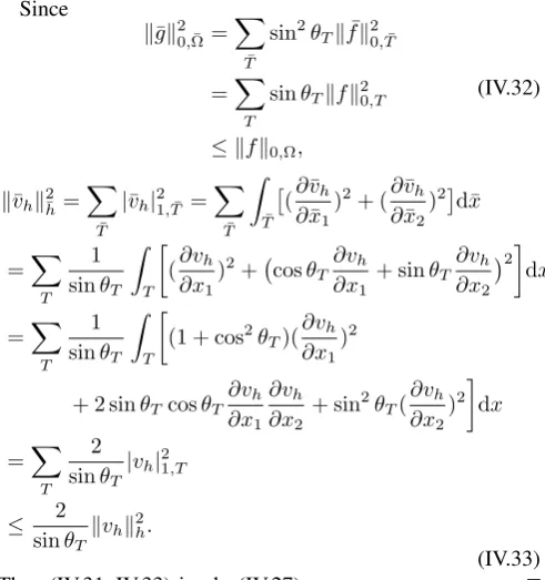
Since

∥¯g∥2_0,Ω¯ =

∑

¯ T

sin2θT∥f¯∥20,T¯

=∑ T

sinθT∥f∥20,T

≤ ∥f∥0,Ω,

(IV.32)

∥v¯h∥2¯_h=

∑

¯ T

|¯vh|2_1,T¯ =

∑

¯ T

∫

¯ T

[

(∂v¯h ∂x¯1

)2+ (∂v¯h ∂x¯2

)2]d¯x

=∑ T

1 sinθT

∫

T

[

(∂vh ∂x1

)2+(cosθT ∂vh ∂x1

+ sinθT ∂vh ∂x2

)2] dx

=∑ T

1 sinθT

∫

T

[

(1 + cos2θT)( ∂vh ∂x1

)2

+ 2 sinθTcosθT ∂vh ∂x1

∂vh ∂x2

+ sin2θT( ∂vh ∂x2

)2

]

dx

=∑ T

2 sinθT|

vh|21,T

≤ 2

sinθT

∥vh∥2h.

(IV.33) Thus (IV.31–IV.33) imply (IV.27).

V. EXPLICIT ERROR ESTIMATE FOR THE MODEL PROBLEM

In sections III and IV, we have explicitly estimate the ap-proximation error and the consistency error for the Crouzeix-Raviart element, respectively, seeing (III.10) and (IV.27). Therefore, according to (II.4) we have the following error estimate for the model problem.

Theorem 5.1: Let u be the solution of (II.3) and uh the

finite element solution defined by (II). Assume θ is the maximal angle. Then the finite element error can be explicitly estimated by

u−uh_h≤

[

2√2C0+

√

2C1

√

sinθ + 4

√

C2 0+

√

2C0

√

sinθ ·(√C2

1+

√

2C1+

√_√

2C2 1+ 4C1

)]

hf_0,Ω,

whereC0≤ 1

π and0.49282≤C1≤0.49293.

VI. NUMERICAL EXPERIMENT

In this section, we test the error bound studied in the above sections by numerical computation. Consider the following Dirichlet problem:_{

−∆u=f, inΩ, u= 0, on∂Ω,

whereΩ = [0,1]×[0,1]andf(x, y) = 2π2_{sin(πx) sin(πy).}

The exact solution of this problem is u(x, y) = sin(πx) sin(πy).

We firstly subdivide Ω into n2 _{small rectangles, where}

each edge of Ω is divided into n segments with n+ 1

points (1−cos(iπ_n))/2, i = 0,1, . . . , n. By dividing each small rectangle into two triangles, we obtain an anisotropic triangular mesh, seeing Fig. 2 (n = 16). Let uh be the

numerical solution.

[image:6.595.48.294.58.320.2]

Numerical calculations are carried out by employing the non-conforming Crouzeix-Raviart finite element method. Nu-merical results are listed in Table 1. Herein,

Fig. 2. An mesh forn= 16.

TABLE I

NUMERICAL RESULTS FOR THE NON-CONFORMINGCROUZEIX-RAVIART FINITE ELEMENT METHOD

n h c ∥u−uh∥h ∥f∥0,Ω C

8 0.270598 5.685837 0.395260 9.869604 0.147999 16 0.137950 10.729399 0.200933 9.869604 0.147581 32 0.069309 20.892908 0.100884 9.869604 0.147481 64 0.034696 41.254045 0.050495 9.869604 0.147458 128 0.017353 81.992482 0.025256 9.869604 0.147462

h= maxThT, C= ∥

u−uh∥h h∥f∥0,Ω

, c= maxT hT ρT

,

wherehT is the diameter of T andρT the diameter of the

biggest ball contained inT.

From the numerical results we can easily see that the ex-perimentally determined constants are below the theoretical estimate (≤8.997472183) given in section V and the error constant is independent of the ratiohT/ρT.

VII. CONCLUSION

We have developed the explicit error estimate for the non-conforming Crouzeix-Raviart finite element based on a careful exploration. The explicit constants of some inequali-ties, together with the consistency error constant, have been obtained. These estimates allow us to derive some com-putable upper bounds of the nonconforming finite element errors, which can serve as a posteriori error estimate. Another feature of our error estimates is that we do not need to assume any mesh condition on the triangulation.

REFERENCES

[1] M. Xie, H. Xie and X. Liu, “Explicit lower bounds for Stokes eigenvalue problems by using nonconforming finite elements,”Japan Journal of Industrial and Applied Mathematics, vol. 35, no. 1, pp. 335–354, 2018. [2] P. L. Lederer, C. Merdon and J. Sch¨oberl, “Refined a posteriori error estimation for classical and pressure-robust Stokes finite element methods,”Numerische Mathematik, vol. 142, no. 3, pp. 713–748, 2019. [3] M. Zhao, H. Guan and P. Yin, “A stable mixed finite element scheme for the second order elliptic problems,”IAENG International Journal of Applied Mathematics, vol. 46, no. 4, pp. 545-549, 2016.

[4] S. C. Brenner and L. R. Scott, “The mathematical theory of finite element methods,” Springer Science & Business Media, New York, 2007.

[5] I. Babuˇska and A. K. Aziz, “On the angle condition in the finite element method,”SIAM J. Numer. Anal., vol. 13, no. 2, pp. 214–226, 1976. [6] E. Carrera, M. Cinefra and G. Li, “Refined finite element solutions for

anisotropic laminated plates,”Composite Structures, vol. 183, no. 2, pp. 63–76, 2018.

IAENG International Journal of Applied Mathematics, 50:1, IJAM_50_1_16

[7] S. C. Chen and L. C. Xiao, “Interpolation theory of anisotropic finite elements and applications,”Science in China Series A: Mathematics, vol. 51, no. 8, pp. 1361-1375, 2008.

[8] D. Guignard and F. Nobile, “A posteriori error estimation for the stochastic collocation finite element method,” SIAM Journal on Nu-merical Analysis, vol. 56, no. 5, pp. 3121–3143, 2018.

[9] N. Kopteva, “Logarithm cannot be removed in maximum norm error estimates for linear finite elements in 3D,”Mathematics of Computation, vol 88, no. 318, pp. 1527–1532, 2019.

[10] K. Kobayashi and T. Tsuchiya, “A priori error estimates for Lagrange interpolation on triangles,”Applications of Mathematics, vol. 60, no. 5, pp. 485–499, 2015.

[11] Y. H. Bai, Y. K. Wu and X. P. Xie, “Superconvergence and recovery type a posteriori error estimation for hybrid stress finite element method,”Science China Mathematics, vol. 59, no. 9, pp. 1835–1850, 2016.

[12] S. P. Mao and Z. C. Shi, “On the interpolation error estimates forQ1

quadrilateral finite elements,”SIAM J. Numer. Math., vol. 47, no. 1, pp. 467–486, 2008.

[13] S. P. Mao and Z. C. Shi, “Explicit error estimates for mixed and non-conforming finite elements,” Journal of Computational Mathematics, vol. 27, no. 4, pp. 425–440, 2009.

[14] F. Kikuchi and X. Liu, “Estimation of interpolation error constants for theP0andP1 triangular finite elements,”Comput. Methods Appl. Mech. Engrg., vol. 196, no. 37–40, pp. 3750–3758, 2007.

[15] T. Apel, S. Nicaise and J. Sch¨oberl, “Crouzeix-Raviart type finite elements on anisotropic meshes,” Numer. Math., vol. 82, no. 2, pp. 193–223, 2001.

[16] A. Maugeri, D. K. Palagachev and L. G. Softova, “Elliptic and parabolic equations with discontinuous coefficients,”Berlin: Wiley-Vch, 2000.

[17] C. Miranda, “Partial differential equations of elliptic type,” Springer-Verlag, 2013.

[18] R. E. Barnhill and C. H. Wilcox, “Computable error bounds for finite element approximations to the Dirichlet problem,”Rocky Mountain J. Math., vol. 12, no. 3, pp. 459–470, 1982.

IAENG International Journal of Applied Mathematics, 50:1, IJAM_50_1_16