Sample Size Determination for Kernel Regression
Estimation Using Sequential Fixed-Width
Confidence Bands
L. Sandamali Dharmasena
∗P. Zeephongsekul
†Basil M. de Silva
‡Abstract—We consider a random design model based on independent and identically distributed pairs of observations (Xi, Yi), where the regression
function m(x) is given by m(x) = E(Yi|Xi = x) with
one independent variable. In a nonparametric setting the aim is to produce a reasonable approximation to the unknown function m(x) when we have no precise information about the form of the true density, f(x)
of X. We describe an estimation procedure of non-parametric regression model at a given point by some appropriately constructed fixed-width(2d)confidence interval with the confidence coefficient of at least1−α. Here,d(>0)and α∈(0,1)are two preassigned values. Fixed-width confidence intervals are developed using both Nadaraya-Watson and local linear kernel esti-mators of nonparametric regression with data-driven bandwidths. The sample size was optimized using the purely and two-stage sequential procedures together with asymptotic properties of the Nadaraya-Watson and local linear estimators. A large scale simulation study was performed to compare their coverage accu-racy. The numerical results indicate that the confi-dence bands based on the local linear estimator have the better performance than those constructed by us-ing Nadaraya-Watson estimator. However both esti-mators are shown to have asymptotically correct cov-erage properties.
Index Term—Nonparametric regression, random
de-sign, Nadaraya-Watson estimator, Local linear esti-mator, fixed-width confidence interval, purely sequen-tial procedure, two-stage sequensequen-tial procedure
1
Introduction
Suppose that (X1, Y1), ...,(Xn, Yn) is a sequence of
in-dependent and identically distributed (i.i.d.) bivariate random variables having an unknown continuous proba-bility density functionfXY(x, y) and without loss of
gen-erality we assume that Xi ∈ (0,1) with a probability
distribution functionfX(x). Consider the nonparametric
regression model
∗Date:06/07/08. Dept. Maths & Statistics, RMIT University,
Melbourne, Australia Email: [email protected]
†Email: [email protected] ‡Email: [email protected]
Yi=m(Xi) +εi, i= 1, ..., n (1)
where εi is a sequence of iid random variables with
E[εi] = 0,E[εi2] =σ2 andm(·) is an unknown function.
The present article attempts to estimate fixed-width confidence bands for the unknown function m(x) at a given pointx=x0. Estimation is based on kernel type
es-timators and consider two most popular kernel eses-timators namely, Nadaraya-Watson estimator ˆmN W,hn(x0) and
lo-cal linear estimator ˆmLL,hn(x0) (Wand and Jones (1995))
which are defined respectively by
ˆ
mN W,hn(x0) =
Pn
i=1yiK(x0h−nxi)
Pn
j=1K(
x0−xj
hn )
(2)
and
ˆ
mLL,hn(x0) =
Pn
i=1wiYi
Pn
i=1wi
(3)
where
wi=K
x
0−xi
hn
(sn,2−(x0−xi)sn,1) (4)
with
sn,l= n
X
i=1
K
x
0−xi
hn
(x0−xi)l, l= 1,2 (5)
hereK(·) is the kernel function andhn is the bandwidth.
In this paper, as in Isogai (1987), we take hn =n−r for
a < r < b; a, b∈ R. As shown above both estimators are weighted averages of the response variable Y. Let
K(·) satisfyR
uK(u)du= 0,R
u2K(u)du≤ ∞,K(u) and
|uK(u)| are bounded. Commonly used kernel functions are listed in Table 1.
Table 1: Selected Kernel Functions
Kernel K(u)
Epanechnikov 3
4(1− 1
5u 2
)/√5 for|u|<√5
0 otherwise
Biweight 15
16(1−u 2
)2
for|u|<1
0 otherwise
Double Exponential 1
2exp(−|u|) for|u|<1
0 otherwise
Gaussian 1
√
2πexp(−(1/2)u 2
) |u|<∞
Uniform 1
2 for|u|<1
0 otherwise
given evidence of continuing interest in the Nadaraya-Watson estimator. One of the strengths of this estima-tor certainly consists in its automatic adaptation to de-signs where the local polynomial estimator may not be performing reliably over all. Also, the Nadaraya-Watson estimator retains some optimality properties as demon-strated in Hardle and Marron (1985).
Methods for obtaining confidence bands form(x) can be found in Hall and Titterington (1988), Eubank and Speckman (1993) and Diebolt (1995). The most widely used confidence band for m(x) is based on the theorem of Bickel and Rosenblatt (1973) for kernel estimation of a density function. Bias-corrected confidence bands for general nonparametric regression models are consid-ered by Xia (1998). In principle, confidence intervals can be obtained from asymptotic normality results for ˆm(x). However, the limiting bias and variance depend on un-known quantities which have to be estimated consistently in order to construct asymptotic confidence intervals.
Sequential analysis, in general, comes in handy when the experimenter’s objective is to control the error of es-timation at some preassigned level. Whether one wants to estimate m(x) at one single pointx0or for all x∈R,
depending on the specific goal and error criterion, one would like to determine the sample size nin an optimal fashion. That is, in order to have the error controlled at a preassigned level, sample size has to be adaptively esti-mated in the process by a positive integer valued random variableN where the event [N =n] will depend only on (X1, Y1), ...,(Xn, Yn) for all n≥1. Finallym(x) is
esti-mated by ˆmLL,hN(x) and ˆmN W,hN(x) constructed from
(X1, Y1), ...,(XN, YN).
2
Nonparametric Kernel Regression
Throughout the present work, we will consider the fol-lowing regression model with a random design. Let
m(x) =E[Y|X =x] (6)
be the unknown regression function which describes the dependance of the so-called response variable Y on the value of X. The following assumptions are used in this study (Wand and Jones (1995)):
(i)m′′(x) is continuous for allx∈[0,1].
(ii) K(x) is symmetric about x = 0 and supported on [−1,1].
(iii)hn→0 andnhn → ∞asn→ ∞.
(iv) The given pointx=x0must satisfyhn< x0<1−hn
for alln≥n0where n0is a fixed number.
The obvious problem that occurs when using (2) and (3) is the choice of bandwidth, hn. According to the
assumption (iii) listed above, bandwidthhnis a sequence
satisfying hn → 0 and nhn → ∞ as n → ∞. Since
we take hn = n−r;a < r < b a, b ∈ R, n−r → 0 and
n1−r → ∞as n → ∞which result in 0 < r < 1. And the assumption (iv) ensures the given pointx0which the
estimation is taking place is selected in such a wayx0 is
more than a bandwidth hn away from the boundary to
avoid boundary effects that ishn< x0 andx0<1−hn.
Combining these assumptions a range of values which r
takes will be decided as shown below:
hn < x0 and hn < 1−x0 ⇔ hn < min{x0,1−x0}
which implies
r >
−ln [min (x0,1−x0)]
lnn
=r0. (7)
Since 0 < r < 1, the above must imply r ∈
(max{0, r0},1) = (rmin,1) where we let rmin =
max(0, r0).
A natural way of constructing a confidence band for
m(x) is follows. Suppose that ˆmq,hn(x) is an estimator
ofm(x) whereq=N W for (2) estimator,q=LLfor (3) estimator then a 100(1−α)% confidence band is of the form
P r{|mˆq,hn(x)−m(x)| ≤d} ≥1−α ∀x∈[0,1] (8)
There are many difficulties with finding a good solu-tion to (8). Firstly, we must derive the asymptotic distri-bution of ˆmq,hn(x)−m(x); secondly we must estimate the
residual variance and distribution function ofX. Also, a good estimator of bandwidthhn is needed.
The kernel estimators are asymptotically normal, as was first shown in Schuster (1972).
Theorem 1. Let K(·) satisfy R
uK(u)du = 0,
R
u2K(u)du ≤ ∞, K(u) and |uK(u)| are bounded, h
n
is such that limnh3
n = ∞ and limnh5n = 0.
Sup-pose x1, ..., xk are distinct points and g(xi) > 0 for
i = 1,2, ..., k. If E[Y3] is finite and if g′, w′, v′, g′′
and w′′ exist and bounded where g(x) = R
f(x, y)dy,
w(x) = R
yf(x, y)dy and v(x) = R
respec-tively, then
p
nhn(mhn(x1)−m(x1), ..., mhn(xk)−m(xk))
d →Z∗
(9) where Z∗ is multivariate normal with mean vector 0
and diagonal covariance matrix C = [Cii] where Cii =
Var[Y|X=xi]R K2(u)du/g(xi) (i= 1, ..., k).
In general the asymptotic bias of the ˆmLL,hn(x)
esti-mator is smaller than ˆmN W,hn(x) estimator (11):
Biasq =E[ ˆmq,hn(x0)]−m(x0) (10)
where
Biasq =
(
A+h2nµ2(K)m′(x)f′(x) f(x) +o(h
2
n) if q=NW
A+o(h2
n) if q=LL
(11)
as n → ∞ where A = h2n
2 m′′(x)µ2(K) and
µ2(K) =R∞−∞u2K(u)du.
However, both estimators have the same asymptotic variance which is
Var[ ˆmq,hn(x0)] = Bσ2
nhnf(x)
+o
(nhn)−1
as n→ ∞whereB=R−∞
∞ K
2(u)du.
Hence in the univariate case of Theorem 1 we have
p
nhn[ ˆmq,hn(x)−m(x)]∼N
0,Bσ
2
f(x)
which leads to
ˆ
mq,hn(x)−m(x) σqf(xB)nhn ∼
N(0,1) asn→ ∞. (12)
3
Sequential
Fixed-Width
Confidence
Interval
Given d(> 0) and α ∈ (0,1) with hn =n−r for r ∈
(rmin,1), suppose we wish to cliam
P {m(x)∈In= [ ˆmq,hn(x)±d]} ≈1−α (13)
which we can rewrite as
P
ˆ
mq,hn(x)−m(x)
p
Var[ ˆmq,hn,n(x)]
<p d
Var[ ˆmq,hn(x)]
!
≥1−α
(14) for largenwherexis fixed.
Using (14) one can see that the probability require-ment (13) leads to the implicit solution-equation
n≥nopt=
(
BZ2
α/2σ2
d2f(x)
)1−1r
(15)
whereZαis the 100%αupper percentile of the standard
normal distribution.
3.1
Purely Sequential Procedure
In general σ2 in (15) is unknown and purely
se-quential procedure suggest to substitute the variance parameter σ2 by a estimator ˆσ2
n0 based on a sample
(X1, Y1), ...,(Xn0, Yn0) of size n0 < nopt. Here we use
the residual variance estimate of σ2 proposed by Ursula
et.al. (2003) based on covariate matched U-statistics:
ˆ
σ2=
P P
i6=j12(Yi−Yj) 2 1
2
1 ˆ
gi−ˆgj
KXi−Xj
hn
n(n−1)
where
ˆ
gi= 1
n−1
X
i6=j
K
X
i−Xj
hn
(16)
and
ˆ
σ2= 1
n
n
X
i=1
ε2i +op(n− 1
2) (17)
Hence from the optimal sample sizenopt given in (15)
we continue sampling until
n≥
(
Z2
α/2Bσˆn2
d2f(x)
)1−1r
(18)
where ˆσ2
n is residual variance estimator ˆσ2based on
sam-ple size n. By taking n = n0 we propose the following
stopping rule for purely sequential procedure which is given by
N = max
n,
(
Zα/2 2Bσˆ2n
d2f(x)
)1−1r
+ 1
(19)
where⌊n⌋refers to the floor function.
In purely sequential procedure we take one observation at a time until the condition given in (18) is satisfied and steps involved in this procedure are as follows:
Step 1: Take an initial sample of size n0, that is select
{(X1, Y1), ...,(Xn0, Yn0)} where Yi is the observed value
ofm(Xi) atXi fori= 1, ..., n0.
Step 2: Now letn=n0 and calculate
(
Z2
α/2Bσˆ2n
d2f(x)
Step 3: Comparenwith
Zα/2 2Bˆσ 2
n
d2f(x)
1−1r
. If
n≥
(
Z2
α/2Bσˆn2
d2f(x)
)1−1r
then final sample size N equals to ni.e. N =n and no further observations are required and hence the process terminates. Go to step 5. Otherwise go to step 4.
Step 4: If (18) is not satisfied increase sample size by one that is new sample size is n0+ 1 and letn=n0+ 1. Go
to step 3.
Step 5: Use the sample{(X1, Y1), ...,(XN, YN)}to
com-pute ˆmN W,hN(x0) and ˆmLL,hN(x0) estimates for m(x0)
and hence construct the confidence band given by (8).
3.2
Two-stage Sequential Procedure
The above purely sequential procedure involves a lot of computational effort. Stein (1945) introduced a sampling procedure which requires only two sampling operations. However, it turned out that this two-stage procedure is less efficient than the purely sequential procedure. Using the asymptotic normality results in the Theorem 1 for univariate random design case we can write
√
nhn{mˆq,hn(x)−m(x)} σp
B(f(x))−1 →N(0,1) (20)
From (17) for a random sample of normally distributed residuals{εi}ni=1 with mean 0 and varianceσ2
nˆσ2
σ2 ∼χ 2
n (21)
whereχ2nis the chi-squared distribution withndegrees of
freedom. Hence we combine (20) and (21) to claim that
√
nhn{mˆq,hn(x)−m(x)}
σ√B(f(x))−1
q
ˆ
σ2 σ2
∼tn. (22)
The following statement (23) is obviously equivalent to (13)
P r{m(x)∈In} ≈t
√ nhnd
p
B(f(x))−1σˆ
! −t −
√ nhnd
p
B(f(x))−1σˆ
!
= 2t √
nhnd
p B(f(x))
!
−1 (23)
where t(·) is the cumulative student-t distribution and an approximate solution to the problem is provided by taking the smallest integern≥1 such that
2t
√
nhnd
p
B(f(x))−1σˆ
!
−1≥1−α (24)
and sincehn=n−r
n≥ t
2
n,α/2Bσˆ2
d2f(x)
!1−1r
(25)
where tn,α/2 =t−1(1−α/2) the (1−α/2)thquantile of
the student-t distribution functiont(·).
Two-stage sampling procedure is initiated by taking a pilot bi-variate sample of sizen0i.e. {Xi, Yi}ni=10 and then
estimate the required final sample sizeN. Now using (25) we propose the following stopping rule for a two-stage procedure
N ≡N(d) = max
n0,
t2
n0,α/2Bσˆ
2
n0
d2f(x)
!1−1r1
+ 1
(26) where r1 ∈ (rmin,1) and from (7) rmin =
max(0,−ln[min(x0,1−x0)]/ln[n0])
If N = n0 then we need no more observations
in the second stage. However, if N > n0 then we
take additional bivariate sample {Xi, Yi}Ni=n0+1 of size
N − n0 in the second stage. Finally we use the
sample {(X1, Y1), ...,(XN, YN)} to compute
Nadaraya-Watson (2) and local linear (3) estimates for m(x0) and
construct the confidence band given in (13). In an appli-cation of the stopping rule (26), it is important to select the best available values for the design constantsr1 and
n0 for fixed predesigned values ofdandα.
4
Simulation Results
We use the following two models to assess the perfor-mance of the confidence bands developed in Section 3: Model I :Y =√4x+ 3 +ǫ
Model II:Y = 2 exp{−0.x182}+ 3 exp{− (x−1)2
0.98 }+ǫ
whereǫ∼N(0, σ2) .
Widths of the intervald= 0.05,0.07,0.09,0.11,0.13 were used. The initial sample sizen0 andσwere chosen to be
25 and 0.5 respectively. The confidence bands were inves-tigated forα= 0.05. For all the data analysed, we used standard normal kernelK(u) = (2π)−1/2exp(−u2/2) and
hence
B=
Z ∞
−∞
K2(u)du=
Z ∞
−∞
1 2πe
−u2
du= (2√π)−1.
In both models 15000 replicate samples for each experi-mental setting were carried out to obtain the final sample sizes required to estimatem(x) atx0= 0.306 given
fixed-width, 2d.
We obtained 15000 random samples of {Xi}25i=1 from
uniform distribution and then calculate correspondingyi
for each stated relation (Models I and II). Random errors
to the above yi to obtained Yi. First we consider
two-stage sequential procedure for α= 0.05 and then purely sequential procedure. The average final sample size ¯n, av-erage residual variance estimate ˆσ2, average local linear
ˆ
mLL,hN, average Nadaraya-Watson ˆmN W,hN estimates
and coverage probability ˜pwhich is the proportion of the confidence intervals that contains the theoretical value,
m(x0) estimated at the pointx0= 0.306 are reported in
Tables 2 and 3 forα= 0.05. In Tables 2 and 3, figures enclosed in brackets under estimated values refer to their standard errors of the corresponding estimated value.
The following are further definitions of the statistics which head some of the columns in the tables:
• ¯n=
Pnsim
j=1 (N)j
nsim
where (N)j is final sample size given in either (26) or
(19) depending on the sequential procedure being used, calculated fromjthsimulated sample andn
sim(= 15000)
is number of simulated samples.
• SE¯n=
r
Pnsim
j=1 ((N)j−n¯)2
(nsim−1)nsim
• %Over= ((¯n−nopt)/nopt) 100%
• mˆLL,hN(x0) =
1
nsim
Pnsim
j=1 ( ˆmLL,hN(x0))j
• SEmˆ
LL,hN(x0)=
r
Pnsim
j=1 (mˆLL,hN(x0))j−mˆLL,hN(x0)) 2
nsim(nsim−1)
where ( ˆmLL,hN(x0))j is the estimated value of local
linear estimator forjthsimulated sample.
• mˆN W,hN(x0) =
1
nsim
Pnsim
j=1 ( ˆmN W,hN(x0))j
• SEmˆ
N W,hN(x0)=
r
Pnsim
j=1 (mˆN W,hN(x0))j−mˆN W,hN(x0)) 2
nsim(nsim−1)
where ( ˆmN W,hN(x0))jis the estimated value of
Nadaraya-Watson estimator forjthsimulated sample.
• ˆσ2= 1
nsim
Pnsim
j=1 (ˆσ2)j
• SEˆσ2 =
1
nsim−1
Pnsim
j=1
(ˆσ2)
j−ˆσ2
21/2
where (ˆσ2)
j is the estimated value of local linear
estima-tor forjthsimulated sample.
• p˜LL=
nmLLˆ (x0 ) nsim
where nmˆLL(x0) is the number of local linear fixed with
confidence intervals that contain m(x0) among nsim
confidence intervals in other words number of confidence intervals which satisfied|mˆLL,Nj(x0)−m(x0)|< dwhere j= 1, ..., nsim
• SEp˜LL =
q
˜
pLL(1−p˜LL)
nsim
• p˜N W =
nmNWˆ (x0 ) nsim
where nmˆN W(x0) is the number of local linear fixed with
confidence intervals that contain m(x0) among nsim
confidence intervals in other words number of confidence intervals which satisfied |mˆN W,Nj(x0) − m(x0)| < d
wherej = 1, ..., nsim
• SEp˜N W =
q
˜
pN W(1−p˜N W)
nsim
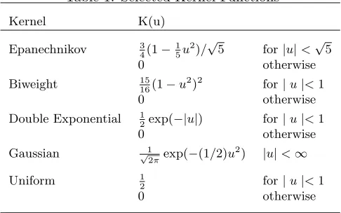
Coverage probabilities of both Nadaraya-Watson (˜pN W) and local linear estimators (˜pLL) have achieved
preset confidence coefficient 95% atx0=.306 in Model II
except when d=.13. But the coverage probabilities for Model I shows a different picture as Nadaraya-Watson estimator fails to achieve required coverage probabilities except when d=.05 where as local linear method does. This noticeable difference is mainly due to structural dif-ferences in the selected models and to the bias terms which heavily depend on derivatives of the unknown func-tionm(·) associated with each estimator. ˜pN W of Model
I is increasing with decreasingddue to large sample sizes resulted in increase in sample sizes. This is consistent with both sequential procedures i.e. two-stage and purely sequential. The performance of Nadaraya-Watson esti-mator worsens asxincreases as its bias highly depends on derivatives ofm(·). For the interior pointx0=.306, the
Nadaraya-Watson estimator assigns symmetric weights to both sides of x0 = .306. For a random design this will
overweigh the points on right hand side and hence create large bias. In other words Nadaraya-Watson estimator is not design-adaptive. However local linear method as-signs asymmetrical weighting scheme while maintaining the same type of smooth weighting scheme as Nadaraya-Watson estimator. Hence local linear method adapts au-tomatically to this random design.
Table 2: Empirical coverage of LL and NW for Model I
α=.05; m(x0) = 2.055
d nopt n¯ p˜LL p˜N W mˆLL mˆN W σˆ2
Two−stage Procedure
.13 81.8 109.3 .947 .902 2.046 2.108 .265 (.40) (.00) (.00) (.001) (.001) (.001) .11 139.0 185.9 .965 .912 2.048 2.105 .262 (.69) (.00) (.00) (.000) (.000) (.001) .09 262.8 340.0 .978 .921 2.048 2.099 .260 (1.28) (.00) (.00) (.000) (.000) (.000) .07 583.6 776.7 .989 .932 2.047 2.091 .265 (2.83) (.00) (.00) (.000) (.000) (.000) .05 1698.2 2259.7 .996 .958 2.048 2.076 .265 (8.34) (.00) (.00) (.000) (.000) (.000)
Purely Sequential Procedure
.13 81.8 80.1 .918 .869 2.046 2.219 .242 (.00) (.00) (.00) (.001) (.001) (.001) .11 139.0 137.6 .954 .901 2.046 2.189 .246 (.00) (.00) (.00) (.001) (.001) (.001) .09 262.8 261.1 .980 .914 2.047 2.109 .248 (.00) (.00) (.00) (.000) (.000) (.000) .07 583.6 581.7 .991 .926 2.047 2.097 .249 (.00) (.00) (.00) (.000) (.000) (.000) .05 1698.2 1695.6 .998 .947 2.051 2.081 .250 (.00) (.00) (.00) (.000) (.000) (.000)
[image:6.612.47.299.87.311.2]it needs significantly more computational times than the two-stage procedure, particularly for small d. However purely sequential procedure at times fall somewhat short of the optimal sample size. Hence the coverage proba-bility falls short of the target, especially when the half width of the interval d becomes larger as this result in smaller sample sizes.
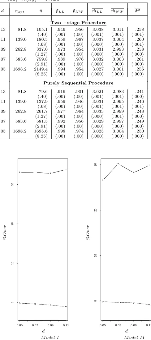
Figure 4.0 reflects the amount of over/under sam-pling (%Over) of average sample sizes ¯nfrom correspond-ing optimal sample sizes nopt based on confidence
in-tervals constructed using two-stage sequential procedure and purely sequential procedure for each half with of the interval d. Average sample size ¯n from two-stage sam-pling method is over samsam-pling whereas ¯ncomputed from purely sequential procedure is slightly undersampling. In practice, the focus is on final sample size, ¯nto be as close as possible to optimal sample size,noptwith a reasonable
coverage probability. Therefore, we can conclude that confidence intervals based on purely sequential procedure has fulfilled the required goal of this study.
Table 3: Empirical coverage of LL and NW for Model II
α=.05; m(x0) = 3.024
d nopt n¯ p˜LL p˜N W mˆLL mˆN W σˆ2
Two−stage Procedure
.13 81.8 105.1 .946 .956 3.038 3.011 .258 (.40) (.00) (.00) (.001) (.001) (.001) .11 139.0 180.5 .959 .967 3.037 3.004 .260 (.68) (.00) (.00) (.000) (.000) (.001) .09 262.8 337.0 .973 .954 3.031 2.993 .258 (1.27) (.00) (.00) (.000) (.000) (.000) .07 583.6 759.8 .989 .976 3.032 3.003 .261 (2.91) (.00) (.00) (.000) (.000) (.000) .05 1698.2 2149.4 .994 .954 3.027 3.001 .256 (8.25) (.00) (.00) (.000) (.000) (.000)
Purely Sequential Procedure
.13 81.8 79.6 .916 .901 3.021 2.983 .241 (.40) (.00) (.00) (.001) (.001) (.000) .11 139.0 137.9 .959 .946 3.031 2.995 .246 (.68) (.00) (.00) (.001) (.001) (.001) .09 262.8 261.7 .977 .964 3.033 2.999 .248 (1.27) (.00) (.00) (.000) (.001) (.000) .07 583.6 581.5 .992 .956 3.029 2.997 .249 (2.91) (.00) (.00) (.000) (.000) (.000) .05 1698.2 1695.6 .998 .974 3.025 3.004 .250 (8.25) (.00) (.00) (.000) (.000) (.000)
+ + + +
0.05 0.07 0.09 0.11
0
10
20
30
o o o o
+
+ +
+
0.05 0.07 0.09 0.11
0
10
20
30
o o o o
Model I Model II
%
O
v
e
r
%
O
v
e
r
[image:6.612.282.548.87.314.2]d d
5
Conclusions
In this paper we have studied data-driven fixed-width confidence bands for nonparametric regression curve esti-mation using local linear and Nadaraya-Watson estima-tors. Both procedures have been produced the correct asymptotic coverage probabilities. The coverage proba-bility of Nadaraya-Watson method was found to be gen-erally below the preset confidence coefficients. On the other hand local linear method had near-nominal cover-age probabilities in most of the cases. The performance of the purely sequential procedure is better than that of the stage procedure. However operationally, two-stage procedure reduces computational costs associated with the corresponding purely sequential schemes by a substantial margin. The estimated residual variance es-timator also appears to be very close to it’s actual value even for small sample size cases.
References
[1] Boularan, J. and Ferr´e, L. and Vieu P., “Location of particular points in nonparametric regression analy-sis,”Australian Journal of Statistics, V37, pp. 161-168, 1995.
[2] Bickel, P. L. and Rosenblatt, M., “On some global measures of the deviations of density function es-timates.,” Annals of Statistics, V1, pp. 1071-1095, 1973.
[3] Diebolt, J., “A nonparametric test for the regression function: asymptotic theory,”Journal of Statistical Planning Inference, V44, pp. 1-17, 1995.
[4] Einmahl, U. and Mason, D. M., “An emperical pro-cess approach to the uniform consistency of kernel-type function estimators,” Journal of Theoretical Probability, V13, pp. 1-37, 2000.
[5] Eubank, R. L. and Speckman, P. L., “Confidence bands in nonparametric regression,” Journal of the American Statistical Association, V88, N424, pp. 1287-1301, 1993.
[6] Fan, J., “Local linear regression smoothers and their minimax efficiency,” Annals of Statistics, V21, pp. 196-216, 1993.
[7] Fan, J. and Gijbels, I., Local polynomial modelling and its applications, Chapman and Hall, London, 1996.
[8] Ghosh, M., Mukhopadhyay, N. and Sen, P.K., Se-quential Estimation, Wiley, New York, 1997.
[9] Hall, P. and Marron, J. S., “On variance estimation in nonparametric regression,”Biometrika, V77, N2, pp. 415-419, 1990.
[10] Hall, P. and Titterington, D. M., “On confidence bands in nonparametric density estimation and re-gression,”Journal of Multivariate Analysis, V27, pp. 228-254, 1988.
[11] H¨ardle, W. and Marron, J. S., “Optimal bandwidth selection in nonparametric regression function esti-mation,” Annals of Statistics, V13, pp. 1465-1481, 1985.
[12] Isogai, E., “The convergence rate of fixed-width se-quential confidence intervals for a probability density function,”Sequential Analysis, V6, pp. 55-69, 1987a.
[13] Martinsek, A. T., “Fixed width confidence bands for density functions,” Sequential Analysis, V12, pp.169-177, 1993.
[14] Quian, W. and Mammitzsch V., “Strong uniform convergence for the estimator of the regression func-tion under ϕ mixing conditions”, Metrika, V52, pp.45-61, 2000.
[15] Schuster, E. F., “Joint asymptotic distribution of the estimated regression function at a finite number of distinct points”,Annals of Mathematical Statistics, V43, pp. 84-8, 1972.
[16] Ursula, U. M., Schik, A. and Wefelmeyer W., “Esti-mating the error variance in nonparametric regres-sion by a covariate-matched u-statistic,” Statistics, V37, pp. 179-188, 2003.
[17] Wand, M. P. and Jones, M.C., Kernel Smoothing, Chapman and Hall, London, 1995.