The Spatial Variation of Membrane
Potential Near a Small Source of
Current in a Spherical Cell
R. S. EISENBERG and E. ENGEL
From the Department of Physiology, University of California, Los Angeles, California 90024
ABSTRACT A theoretical analysis is presented of the change in membrane potential produced by current supplied by a microelectrode inserted just under the membrane of a spherical cell. The results of the analysis are presented in tabular and graphic form for three wave forms of current: steady, step function, and sinusoidal. As expected from physical reasoning, we find that the membrane potential is nonuniform, that there is a steep rise in membrane potential near the current microelectrode, and that this rise is of particular importance when the membrane resistance is low, or the membrane potential is changing rapidly. The effect of this steep rise in potential on the interpretation of voltage meas-urements from spherical cells is discussed and practical suggestions for mini-mizing these effects are made: in particular, it is pointed out that if the current and voltage electrodes are separated by 600, the change in membrane potential produced by application of current is close to that which would occur if there were no spatial variation of potential. We thus suggest that investigations of the electrical properties of spherical cells using two microelectrodes can best be made when the electrodes are separated by 60°.
The electrical properties of spherical cells are often investigated by inserting two microelectrodes just under the cell membrane. One electrode, the current or source electrode, is used for passing current; the other, the voltage or re-cording electrode, for rere-cording potential (Fig. 1). It is usual to assume that the change in membrane potential produced by passing current is quite inde-pendent of the angular separation of the electrodes (Eccles, 1957; Rall, 1959, has further references; Hellerstein, 1968) since the radii of spherical cells are in general much smaller than the length constant of cylindrical cells. That is to say, if a cylindrical cell had the same diameter and were made of the same material as a spherical cell, the potential along the cylindrical cell would not change appreciably in distances comparable to the radius of the spherical cell. However, recent analyses of the three-dimensional spread of current near a
736
The Journal of General Physiology
on May 2, 2019
jgp.rupress.org
Downloaded from
http://doi.org/10.1085/jgp.55.6.736
R. S. ESENBERG AND E. ENGEL Spatial Variation of Membrane Potential
point source (in practice, a source very small compared to the dimensions of the cell) in a cylindrical cell (Falk and Fatt, 1964; Eisenberg, 1967; Adrian, Costantin, and Peachey, 1969; Eisenberg and Johnson, 1970) as well as in a thin plane cell and a thick plane cell (Eisenberg and Johnson, 1970) have shown that, sufficiently near a point source, there is a steep rise in true trans-membrane potential not predicted by the usual one-dimensional theory. The physical origin of this steep rise in potential is that in the neighborhood of a point source, the current density is very high. Since the resistance of this region is not zero (indeed the resistance of this region is very high because of its small dimensions) the potential near the source must be very high. This phenome-non is analogous to the familiar "convergence resistance" (that is, the re-sistance associated with the flow of current from a small source imbedded in an infinite resistive solid) although the presence of a high resistance membrane greatly complicates the analysis of the biological case. Since the physical cause of this steep rise in potential lies in the size and shape of the source, not the over-all shape of the membrane (provided the membrane is reasonably smooth near the source), a similar phenomenon would be expected to occur in a spherical cell. Indeed, in an early publication Rall (1953) mentioned that such a steep rise (or more precisely, a "singularity") in membrane potential occurs in one of the solutions of an equation for the membrane potential of a spherical cell.
It thus seemed of interest to reinvestigate quantitatively the assumption of the uniformity of membrane potential in a spherical cell, particularly looking for deviations in the region of the point source. Our investigation was made for three types of source; a steady source, a step function source, and a sinu-soidal source. The results of these computations are presented in both tabular and graphic form. The details of the analysis for each case can be found in the appropriate Appendix.
Several conclusions from our analysis may be of interest to the general reader: (a) There is a striking nonuniformity of membrane potential near the point source, and this nonuniformity becomes of particular importance when the membrane potential is changing rapidly or when the membrane resistance is low. (b) A simple equivalent circuit describes, to a first approximation, the effects of the nonuniformity of membrane potential. (c) There is a region of the cell (a ring situated at about 600 from the source) in which the membrane potential is close to the membrane potential of a cell of uniform potential. Measurements made with this angular separation between the current source and voltage electrode can be interpreted, at least to a first approximation, using the usual equations for an isopotential cell. Thus, it seems reasonable to recommend that experimental measurements of the electrical properties of spherical cells be made with an electrode separation of about 60°.
THE JOURNAL OF GENERAL PHYSIOLOGY VOLUME 55 1 I970
RESULTS
The precise problem we wish to solve is the following. What is the change in membrane potential of a spherical cell when a current is applied to the cell from a point source' just under the membrane, assuming the external medium remains isopotential (Fig. 1)? A solution to the problem can be found from Hellerstein (1968) or Carslaw and Jaeger (1959) and can be considerably simplified as shown in Appendix 1. We will first present the steady-state solu-tion and then show how this can be generalized easily to the transient solusolu-tion for a step of current, or the solution for a steady sinusoidal excitation.
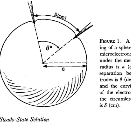
FIGURE 1. A schematic draw-ing of a spherical cell with two microelectrodes inserted just under the membrane. The cell radius is a (cm); the angular separation between the elec-trodes is 0 (degrees or radians); and the curvilinear separation of the electrodes, measured at the circumference of the cell, is S (cm).
Steady-State Solution
The steady-state solution can be written as
vm
=4-
° [ - 2a/A}{1 +- (a/A)D - (a/A)2E}±
(a/A) csc /21 ( I ) whereD n = csc2 0/2 1 ± csc
0/2
E0 = P,(cos) n = 1,2,3,
1 The approximation inherent in describing the microelectrode source as a point is of little signifi-cance. An analysis of the solution for a disc source (E. Engel and R. S. Eisenberg, unpublished data) shows that, as might be expected on physical grounds, when the diameter of the current source is a small fraction of the cell circumference, the spatial variation of potential is substantially the same as that described here. Even when such is not the case, the qualitative features of the spatial variation of potential are similar to those described here.
[image:3.612.150.376.284.494.2]R. S. EISENBERG AND E. ENGEL Spatial Variation of Membrane Potential
and where Vm is the membrane potential; i is the current applied; a is the radius of the spherical cell (units: cm), R, is the resistance of 1 cm2 of mem-brane (units: ohm-cm'), Ri is the volume resistivity (units: ohm-cm) of the cytoplasm, the ratio of these quantities is called the generalized space constant2 (that is, Rm/R = A; units: cm), 0 is the angular separation between the elec-trodes (an angular separation of 0 degrees corresponds to a curvilinear separa-tion of S = a07r/180 0.175 a) and P, is a Legendre polynomial (Abramowitz and Stegun, 1964). It is shown in Appendix 1 that this solution, while not exact, is sufficiently accurate under physiological conditions. Even under worst case conditions when the space constant is twice the radius, the total error in equation (1) is less than 2.2% for all angles. It is interesting to note that, except for a scale factor, equation (1) depends on only two param-eters, the angular separation 0, and the ratio of radius to generalized space constant a/A.
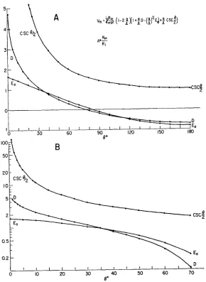
Table I and Fig. 2 give the values of the functions D, Eo, and csc 0/2. It can be seen that for small angular separations and small values of a/A the domi-nant term of equation (1) is (a/A) csc 0/2 and thus an approximate form of the solution is
V.- -~ z {I + (a/A) csc0/2 = - + i csc /2 (3)
0 4ra2 4ra2 47ra
in which the second term has the units of resistance and will later be called
R, (Fig. 6). With Table I it is a simple matter to compute the effect on
mem-brane potential of the three-dimensional spread of current. One determines the value of the generalized space constant A appropriate to the problem; the angular separation 0 of the source and recording electrode; and the radius
a of the cell. Then using equation (1) and the values of D, Eo, and csc 0/2
given in Table I, one can calculate the potential expected at the tip of the voltage electrode.
It is useful to analyze equation (1) in another way. If one remembers that the expression for the membrane potential in an isopotential cell (that is, a cell in which the voltage gradient produced by the three-dimensional spread of current is of no significance) is Vm = iR,/4ira2, then we see that the full
three-dimensional solution consists of the isopotential expression multiplied by a correction factor. In other words this correction factor is the ratio of the potential predicted by three-dimensional theory to that predicted by
isopo-2 It should be pointed out that in this paper the symbol A refers only to the DC generalized space constant. That is to say, A is identical to R,/R iand is entirely independent of capacity current and
thus time. In the qualitative analysis of time-dependent phenomena it is useful to introduce a gener-alized frequency-dependent space constant (see Eisenberg and Johnson, 1970, p. 59) but this is possible here only to the limited extent that equation (3) is an adequate approximation. The reader should be warned that the generalized space constant A is not analogous to the length constant
X = [aR,/2Ri]l defined for long cylindrical cells.
THE JOURNAL OF GENERAL PHYSIOLOGY VOLUME 55 1970
tential theory and thus measures the fractional error in the isopotential expres-sion. The correction factor depends only on the angular separation and the ratio of the radius to space constant. Table II presents values of this correction factor for a wide variety of "space" constants and angular separations. The column headed 60° is set in boldface type since for this electrode separation
TABLE I
THE MEMBRANE POTENTIAL IN A SPHERICAL CELL INCLUDING THE EFFECTS OF THE THREE-DIMENSIONAL SPREAD OF CURRENT
V. = ioI 4iasI -2a/A}II + (a/A)D - (/A)'EoI + (a/A)cc/2]
0 0 5 10 20 30 40 50 60 70 80 90 100 110 120 130 140 150 160 170 180 D o 3.090 2.356 1.591 1.121 0.779 0.509 0.288 0.103 -0.054 -0.188 -0.302 -0.399 -0.480 -0.547 -0.600 -0.641 -0.670 -0.687 -0.693 1.64 1.55 1.45 1.24 1.03 0.82 0.61 0.41 0.23 0.05 -0.11 -0.25 -0.38 -0.50 -0.60 -0.68 -0.74 -0.79 -0.81 -0.82 Co 22.926 11.474 5.759 3.864 2.924 2.366 2.000 1.743 1.556 1.414 1.305 1.221 1.155 1.103 1.064 1.035 1.015 1.004 1.000
A is defined as the ratio of the membrane resistance (ohm-cm2) to the internal resistivity (ohm-cm); i.e., A = R/Ri . a is the cell radius.
0 is the angular separation of electrodes.
The computation was carried to enough figures to ensure that the last significant figure is correct.
the correction term is negligible for all values of a/A considered. Figs. 3 and 4 are graphical representations of the same data. It is clear from these plots that the correction factor becomes significant when a/A is large and/or the elec-trode separation is small. For resting values of the membrane resistance (that is for R, of the order of a few thousand ohm-cm2) and for cell radii in the usual range (from say 0.05 to 0.005 cm) the radius is small compared to the space
740
R. S. EISENBERG AND E. ENGEL Spatial Variation of Membrane Potential
A
Vm (-2AXI+AD -(A 2 CSC)Rmn
Ri
[image:6.612.161.451.131.528.2]60
FIGURE 2. Graphs of the size of the various terms in the equation for the membrane potential at different values of electrode separation. The upper graph (A) is a linear plot showing the general shape of the curves over the whole range of angular separa-tion 0. The lower graph (B) is a plot of the same results with a logarithmic ordinate and over a smaller range of angles.
constant (a/A is around 10- 3) and the effect of the three-dimensional spread of current is small even at electrode separations of 5°. By extrapolation (and indeed by analysis) it can be seen, however, that at sufficiently small separa-tions the correction term is important. Thus, when a single electrode bridge or double-barreled electrodes are used (Eisenberg and Johnson, 1969),3 the 3 Note Added in Proof We have recently derived a precise and surprisingly simple expression for the voltage recorded by a single electrode bridge.
THE JOURNAL OF GENERAL PHYSIOLOGY · VOLUME 55 1970
C0 N O co
-0,. R 9 co co 000000
u) CO - _ U - U D N C0 t _; ts i 8
CO CO CD U l . .D .L NO m . . .CO C 1U0 If) CO~ U~ . OL
000000000000000
_ N N m N -Cw C
Cd C C C . C. . . . CC C CR b L
CD co cc1 g CXX " F Nw O D - - g L O
.. . . .R ...
0 0 CD 0000 b £ 0 CD 0 0 0 CD O 00
LO Cli 0 C 0 0 0 00D - 0 0 00 b 0 0 00 0
O-Co o o o co o Lo o o o o O 0 oo
(3r & ) CO N O
000000000000
o o oo o o o o 0 c ... of.° 0 9.. to
- >0 N = N4 ) I4 -- N r C-0 o t0) co L, N o co 0 ot.t6
C9 c8 .. o c'h
u 0
m CN i Co t; U) N 0 - cO
0-en N - C u -co - co
N-N 0N CO -0
O O - co n
C O OO O O- -N C c C0
... ... ...
- -- - -- - -- -- -- -N N N > C + > _ Q 0 +C 3 0C 0b+eC
-+U')t NX C g _ + s 0 C - N+ eC
o ooo o-- NCO+U' d ddO b -- CJ 1
- ____NN
+ ( O+C0N D O DN +C0N+ N bC C 0 e
N N+ 1 C C -CX+ +C0- + ON -CDQ
O~ O -NN+1CD-+sC
~
-C-
~ ~
~
~
NNNNC -~
·u)>0 · u. 0 . 0 Z O< 0
o9
.q .
e C 0 0 o 0 8 o _so C !2 0 S a 8 1 _ oI o0 0 C. U 4" 00 >0 . w u Cdd * . C ee teo
e *
c O
N o z U 1 C § O mi- Lo " ,~
88 O c0cc U0 1-C0SO
742
I o
-R. S. EISENBERG AND E. ENGEL Spatial Variation of Membrane Potential
_-0. Correction Foci a is Cell Radius
The Value of
\S
'or x 4 = Three-Dimensional Solution ,A, = Rm/Ri
/A For Each Curve is Indicated
01
I I I I I If I I I I
200 400 600 800 1000 1200 1400 1600 1800
FIGURE 3
Correction F
a is Cell Rodi
The Space C
Rm~~~~~~~~~~~~5 'actor x Rm = Three-Dimensional Solution
ius
onstant A = RI
20'
300
40' 50'
70*
900 200 1800
...
I . ... I
0.01 a
A
0.1 0.5
FIGURE 4
FIGURES 3 AND 4. Plots of the correction factor (ordinate) for different conditions of interest. In Fig. 3 the abscissa is the angular separation between electrodes and each curve is labeled with the appropriate value of a/A. In Fig. 4 the abscissa is the value of a/A (on a logarithmic scale) and each curve is labeled with the appropriate value of 0.
correction would be expected to be particularly important. Furthermore, we see that whenever the space constant is comparable to the cell radius the correction factor is significant over a wide range of angles. This latter condi-tion occurs, in effect, when rapidly changing currents are considered, whether
8.0
4.0
2.0
IO
I.C
0.1 0.0101
nn.,
I 1 1111111 1 I 1 111111 111 I I
743
---h.
THE JOURNAL OF GENERAL PHYSIOLOGY · VOLUME 55 1970
they be sinusoidal or of other shape (see below). Finally, under many condi-tions of physiological interest the membrane resistance itself drops to quite low values, sometimes low enough so that the space constant is comparable to the cell radius. It is under these conditions of very small electrode separation, rapidly changing voltages, or low membrane resistance that the correction for the three-dimensional spread of current becomes important.
Transient Solution
In Appendix 2 the transient solution of the three-dimensional problem for a step function of current applied at time t = 0 is given. It is shown there that the terms in the solution which express the dependence of the potential on angular position (the three-dimensional correction terms) are established very quickly compared to the terms which describe the change in potential with time for an isopotential cell: indeed, the time constant which roughly describes the time dependence of the three-dimensional fields is quicker (i.e. smaller) than the membrane time constant RmCm by a factor of (A/a) + 1.
Thus, at times of physiological interest the response to a step function of current is described by (see equation (41) in Appendix 2)
V--- = - ( --e- t mcm)
+
(2a/A) 1 Pn (cos 0) ( 4 )4rwa2 . .,-,n + a/A
which can be simplified, as shown in Appendix 1, to
V. = 4(aI4r 2 {L(t) + (a/A, 0) (55
where r4(a/A, ) determines the spatial variation of potential
i
= I - 2a/A}{1 + (a/A)D - (a/A)2Eo} + [(a/A)csc 0/2] - 1 (6)and L(t) determines the time response of the cell
L(t) = 1 - e-tlRCm (7)
Note that this term is precisely the same as that which describes the response of an isopotential cell to a step function of current. The numerical value of the term, ~4(a/A, 0) the three-dimensional correction term, can be determined by subtracting one from the correction factors previously given (see Table II and Fig. 3). While at the times of interest the absolute value of the three-dimen-sional term
4
is independent of time, the relative importance of this term varies greatly with time depending on the size of the isopotential term L(t). Thus, the relative importance is greatest at short times when the isopotential term is small. A plot of the relative importance of the three-dimensional term (thatR. S. EISENBERG AND E. ENGEL Spatial Variation of Membrane Potential
is a plot of p/L) is given in Fig. 5, where an inset shows the wave form of the time response and a schematic definition of
4,6
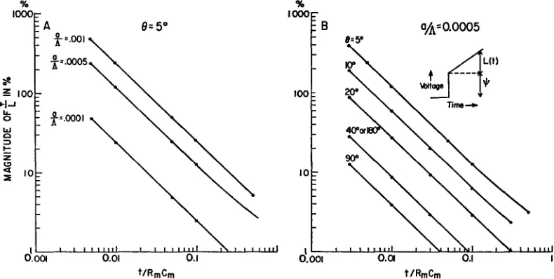
and L. It can be seen that the three-dimensional effect is of significance primarily for small times and small angles. Note that for angular separations of around 600 the three-dimensional term is very small at almost all times, and thus cannot be conveniently shown in this log-log plot.The curves presented in Fig. 5 B would be directly applicable to a cell of
% %
t/RmCm t/RmCm
FIGURE 5. Plots showing the relative importance of the spatial term (0) compared to the isopotential term L(t) as a function of the time following the application of a step function of current. A schematic definition of 1 and L(t) is shown in the upper right-hand quadrant of the figure. A precise definition is found in equations (6) and (7). The left-hand plot (A) was computed for an electrode separation of 50, the values of a/A being indicated beside the appropriate curve. The right-hand plot (B) was computed for a/A = 0.0005, the value of 0 being indicated for each curve. For values of the elec-trode separation near 600 the value of 4/L is so small that it cannot be shown on the logarithmic ordinate.
membrane resistance 2000 ohm-cm2, internal resistance 200 ohm-cm (thus A = 10 cm), and radius 50 #u. If the membrane capacitance were 2 uF/cm2, RC, = 4 msec. Thus, at 40 /isec after the application of a pulse of current, and at an electrode separation of 50, the spatial variation of potential produces a (roughly) 100% effect, at 400 ,sec a (roughly) 10% effect.
DISCUSSION
General Conclusions and Relation to Previous Results
The general conclusion from our analysis is that the change in membrane potential in a spherical cell produced by current applied from a microelectrode
[image:10.612.112.507.243.442.2]THE JOURNAL OF GENERAL PHYSIOLOGY · VOLUME 55 1970
lying just under the membrane is quite uniform around most of the cell, with striking deviations in the vicinity of the microelectrode source. These devia-tions are particularly important under condidevia-tions where there is a high current density crossing the membrane, that is when the membrane resistance is low or during rapid changes in membrane potential.
It is now necessary to discuss why this nonuniformity of potential has been overlooked by previous investigators (however, see Rall, 1953). The solution to a similar but somewhat more general problem has been previously found by Hellerstein (1968) and Eisenberg and Johnson (1970), and as shown in Ap-pendix 1 these solutions coincide at least for the particular case which we consider here, namely with the current electrode just under the membrane. Essentially, the reason that our interpretation of the solutions differs is that we have quantitatively evaluated the solution in the region near the point source, and investigated the convergence properties of the solution in that region. Thus, while the second term in the infinite series (our equation (10) or equa-tion (98), p. 376 of Hellerstein, 1968) is very much smaller than the first term, (even at zero electrode separation), the third (and higher) terms are ap-proximately equal to the second term and thus when sufficient terms are in-cluded the first term is no longer dominant. The above statement is simply a qualitative way of stating that at zero angular separation the infinite series defining the potential does not converge. It is easy to prove this point directly
remembering that P,(1) = 1 and that the sum E (l/n) does not converge; nit is more difficult to show that the other form of the solution (namely, our it is more difficult to show that the other form of the solution (namely, our equation [8]) does not converge, but this can be done. The reason for this failure in convergence and thus, in physical language, the steep rise in poten-tial near the point source, lies in the nature of a three-dimensional point source: a point source forces a finite current to flow through an infinite re-sistance and thus requires an infinite potential (see, for example, Table 1-1, p. 12 of Panofsky and Phillips, 1955).
Effect of Electrode Depth
We have not been able to evaluate the change in membrane potential pro-duced by a current injected from a microelectrode at an arbitrary depth within the cell. The solution derived by Eisenberg and Johnson (1970) is im-practical in this case since it converges exceedingly slowly, and we have not been able to simplify the solution with a theorem analogous to that developed in Appendix 1. Nonetheless it seems quite clear that the essential result of our analysis, namely the existence of a steep rise in membrane potential near a point source, is true even if the source is not immediately under the membrane but is somewhat deeper in the cell. The reason for this conclusion is as follows. Except perhaps right at a source the functions which describe any electric
R. S. EISENBERG AND E. ENGEL Spatial Variation of Membrane Potential
field are continuous functions of distance and have continuous derivatives up to and including at least the second order (this statement is implied by the fact that away from a source an electric field can be described by Laplace's
equation [equation 34]). Thus, as a source is moved from just under the mem-brane deeper into a cell the memmem-brane potential does not change abruptly.
The above abstract reasoning is consistent with the results computed for a cylindrical cell by Eisenberg and Johnson (1970, Pt. A, sect. IV.4) for a prob-lem analogous to ours. They showed that the qualitative features of the spread of potential were the same whether the source was located at r = a or at
r = 0.75 a. Thus, even when the source is quite deep within the cell there is a
steep rise in true transmembrane potential in the vicinity of the electrode.
Physiological Implications4
The discussion of Eisenberg and Johnson (1970, Pt. B, sect. 1, pp. 46-56) con-cerning the physiological implications of the steep rise in membrane potential near a point source of current is applicable to the spherical cell. In particular, the three-dimensional effect is important in understanding (a) the nature of the artifacts produced when potential is recorded with the same microelec-trode that is used for passing current, (b) the artifacts associated with the use of double-barreled microelectrodes, (c) the difficulties involved whenever one seeks to control the membrane potential of a cell with current supplied from a microelectrode.
It is clear that in routine measurements of the electrical properties of spher-ical cells the electrodes should be placed at an angular separation of around 60°; this corresponds to a curvilinear separation of 1.05 a where a is the cell radius. With this separation under conditions of physiological interest, there is almost no deviation of potential from that predicted for an isopotential cell. When the electrode separation is small enough so that the three-dimensional correction is significant, the full equation (1) can be approximated to some extent by equation (3). Thus, the major effect of the three-dimensional spread of current is to produce an additional potential the absolute size of which is independent of the membrane resistance or impedance but whose relative importance does depend on the membrane properties. It should be empha-sized that this extra potential represents a component of the true transmem-brane potential and does not represent an internal potential drop in the re-sistive medium filling the cell. We have seen that the variation in membrane potential drop associated with the three-dimensional spread of current is established very quickly (with a time constant of roughly RiCa = R,C,
{
a/A },see equation [40]) compared to other changes of membrane potential with time. Thus, as a first approximation the main effect of the three-dimensional
4 Note Added in Proof Two papers (Rall, W, 1969. Biophys. J. 9:1483, 1509) have recently
ap-peared which discuss this topic.
THE JOURNAL OF GENERAL PHYSIOLOGY VOLUME 55 1970
Isopotenfial General
Cmx47o2 1 Rm True Rm Cmx4oa2
4T0 t 4jra2 Tronsmembroane r2
CmX~r02O
1
Ryf (9) [image:13.612.169.444.137.214.2]Cell Radius a, Angular Separation of Electrodes 8
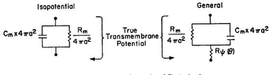
FIGURE 6. The equivalent circuit of the spherical cell. This circuit is most useful in a qualitative sense, since R, has physical meaning only when the electrode separation is small and the space constant is large. More precisely, this circuit is useful when the approximate equation (3) is satisfactory.
spread of current is to produce an additional potential drop across the mem-brane, this potential drop being proportional to current and independent of time. In other words the main effect of the three-dimensional spread of current can be represented by modifying the equivalent circuit of the spherical cell to include a resistance Rp (equivalent to the second term in equation [3]) in series with the usual parallel arrangement of R, and Cm (Fig. 6). The size of this equivalent resistance is given by the various tables and figures in the Results section. It should be pointed out that the resistance Rp has limited physical significance, in that it is a useful description only to the extent that the ap-proximate equation (3) is valid, that is only when the angular separation between electrodes is small and when the generalized space constant A is large.
APPENDIX 1
Part 1. Derivation of the Solution
The full solution to the problem of the membrane potential in a spherical cell, the source of current being a point lying just under the membrane, has been given by Hellerstein (1968) and determined by Eisenberg and Johnson (1970, Pt. A, sect. V) by an integration of a solution presented in Carslaw and Jaeger (1959, p. 382).6 The solution derived by Eisenberg and Johnson is written here in terms of cylindrical Bessel functions Jn + 1/2 and Legendre polynomials P, (see Abramowitz and Stegun,
1964).
V i Ri (2n + )P. (cos ) 1 (a/A
2ra ,n-o .-1 ,)2 (a/A - + 0.2 ( + )2
where P, are the positive roots, numbered in order of increasing magnitude, of
(a/A - )J + (I8) + J' + (.) = 0 (9)
A prime denotes the derivative.
5 The corresponding differential equation and boundary condition are given here in Appendix 2, equations (32) and (33).
R. S. EISENBERG AND E. ENGEL Spatial Variation of Membrane Potential
The solution given by Hellerstein (1968) includes the effects of external resistance and different radial locations of electrodes, but can be specialized to our case by setting r = a, t = oo, and using our names of variables
V i= R , n + i p (cos 0) (10)
2ra n- n + a/A
The first part of this Appendix is devoted to showing that these two solutions coin-cide, the second part of the Appendix then shows how to write the solution in much simpler form.6
It is easy to see that equations (8) and (10) are identical if and only if
1 1
.1
8,2 + h2 _ 2 2(h + v)where h is defined as a/A - ½ and v (any real number) is written to denote the order of Bessel function (which in equation (8) was written as n + 3). It was gratify-ing to find a statement of this relation in Lamb (1884, footnote, p. 273) but the tantalizing absence of a proof made the following derivation necessary. Full details of the proof are given but we refer the reader to works on complex analysis (for example, Whittaker and Watson, 1927; Markushevich, 1965) for the necessary back-ground material.
Our plan of attack will be to consider a function F(z) of Bessel functions closely related to equation (9), namely
F(z) = zJ(z) + , (z) 12)
Note that F(z) has a simple power series expansion which can be derived from the expansions of J,(z) and JI,(z) (Whittaker and Watson, 1927, sect. 17.2):
F(z) = ( +) + h) --_ Z 22 + +2)
2,r' +
1)
2(2 + 2)(13)
+ Z4
4+v
+h
+
(2)(4)(2v + 2)(2v + 4) +
Definitions, properties, and tables of the gamma function r(z) can be found in Abramowitz and Stegun (1964).
We now expand this function F(z) into an infinite product in order to determine the roots f and to derive the desired sum. Since the function F(Z) is well-behaved (that is, it can be differentiated at every point in the complex plane) and has simple (that is, not repeated) roots at the points , it can be written as a Weierstrass infinite 6 The following proof is presented in detail because we were originally skeptical of the equality of the two solutions and felt that a proof was necessary. Moreover, the following proof uses a powerful method which is not found in standard texts and may be useful.
THE JOURNAL OF GENERAL PHYSIOLOGY · VOLUME 55 1 I970
product (Whittaker and Watson, 1927, sect. 7.5) of the form
F(z) = F(0)[exp{zF'(0)/F(0)}] II {(1l - z/1)e"l} (14)
and we have used the standard notation for infinite products (Markushevitch, 1965, p. 334).
IIfs(z) = fxi(z)z)f (z) ... (15)
a-i
Fortunately, in our case this expression can be considerably simplified. We note that in the series expansion of F(z) (equation [13]) all the powers of z are even. Thus, if # is a root of equation (12) so is -A also a root. Then, every factor eP in the infinite product (14) is multiplied by a factor e-1I/ and thus becomes unity. Similarly, the factors (1 - z/#) and (1 + z/l) multiply to give a perfect square and the infinite product expansion takes the form
F(z) = F(O)[exp{zF'(O)/F(0) }] I (1 - 2/,2) (16)
8s1
where the product is taken over all the positive roots 3,, numbered according to size /1 < 2 < -·-. We can evaluate the first two factors in this equation from the power series expansion (13). Thus
lim F(z) - + h and lim F'(Z) = 0 ( 17)
· 0 2'r(' + 1) ,-o F(z)
So we have as the final simplified form of the product expansion
F(z) h z _ = v+h I (1 - z2/ 2
)
(18)In order to convert the infinite product into a sum we take the logarithm of both sides and then differentiate,
J' + (l/z)(l + h)J: - 2
- Z_ - z (19)
zJ, + hJ, Z 2
This relation is beginning to look promising since it gives a closed form expression for an infinite sum involving the roots , . However, a few more manipulations are necessary to put the series in the form we seek. We notice that for a special value of z namely
= zo - (v - h2)t (20)
R. S. EISENBERG AND E. ENGEL Spatial Variation of Membrane Potential
Thus, if we let z = zo in both sides of equation (19), we have
2 v J,' (zo) + (I/zo)J(zo) + (h/zo)J, () (21)
,-1 : - v2 + h2 Zo
4
z. J(z) + U, (z.)
J()
+
hJ()Note that this equation gives a closed form expression for the infinite sum. But the right-hand side of this equation can be considerably simplified by using the differen-tial equation which defines Bessel functions
J + (/z)J + (1 - v2/z2)J, = 0 (22)
If this equation is evaluated at z = zo we have
J '(Zo) + (l/zo)J(zo) = (h2/z,)J,(zo) (23)
Then, we substitute equation (23) into equation (21)
2 __1 P (h/z!)[zoJ(zo) +
h,(z)]
24,-1 8 - v2 + h2 Zo
zoJ;(zo) + hJ,(zo)
cancelling and using equation (20),
1 v-h 1
2 _-1 ~ _ _E_ v + h2 (25)
P2 _ h2 + h
This completes our proof of equation (11) and establishes the identity of the two solutions (8) and (10).
Part 2. Simplification of the Solution and Computational Methods
The solution presented above, while correct, is quite impractical. Since it is an in-finite series which converges slowly (that is to say, which requires the consideration of many terms), it requires a great deal of computation and yields little physical insight. We will now put this solution into more useful form. The plan of attack is to manipulate the series into a form where much of the infinite series can be summed (i.e. written in closed form).
We consider the infinite series alone and perform long division:
.
n +a
p(cosO)= p(cosO) a/AP-(o )E
"
'Pn
(Cos ) =
P
(os )
-
Pn (cos )(26)
n= n + aA n-l n-l + aA
-
Z)
Pn (cos - A_1) I Pn (cos 0)/,,(PO 1
.(cos)
(27)(a/A) a/
-1 n(n + a/A)
THE JOURNAL OF GENERAL PHYSIOLOGY · VOLUME 55 1970
which can be rewritten
±Qo/~)a/A)-lPn(2 o/A) ,,=-
E P
(Cos ) +
a/A E/
-______ 2 1 n -c I6)(28)
+ (a/A) a/A - I (os - (a/A)' a/A -
)
( +a/)The first two of these infinite series can be summed in closed form by simple ma-nipulation of the infinite series which generates Legendre polynomials (see Wheelon, 1968, p. 53):
n y- csc2 /2
P
/ (osO)= -+ -csc /2 + 2-- a/A ln + csc /2
n-1
~~~~~_~aA
\/\/ lcs /2 (29)(a/A)- a) = P, (os6) + (a/ 21 a P, (os6)
I /) n2 (a/A)2 -a/A n2(n + a/A)
Thus, it is only necessary to compute the last two infinite series in equation (29). The first of these infinite series has the useful property that it depends only on the elec-trode separation and is independent of the properties of the cell, namely the radius and the generalized space constant. Thus, this series need be evaluated only once for each angle and yet is still applicable to all cells. This series was summed for those angles shown in Table I on a Hewlett-Packard 9100A desk calculator (which has an accuracy of 10 significant figures) using the tables of P, (cos 0) of Clark and Churchill (1957). Sufficient numbers of terms were used so as to ensure the signifi-cance of the least significant digit in all cases. In no case should the figures be in error by more than 40.005. The sums for = 0° and 1800 are known in closed form, and thus for those cases our summation procedure could be checked.
Since we are concerned only with cases in which the generalized space constant is larger than the cell radius (that is, a/A < 1), the final infinite series in equation (29) would be expected to be relatively insignificant and we will now examine the error involved in ignoring this term. We will consider the sum
(a/A) - a/A P, (os ( 30)
n1 n
8
which is clearly always larger than the sum of interest for a/A < 1. Thus, the error we compute is an upper bound. This sum is largest in magnitude for 0 = 0°, in which case the value of the sum is (since P,(1) = 1) (Wheelon, 1968, p. 7)
(a/A)2 a/A) E 1.202(a/A)2 (1-a/A) (31)
The relative error in equation (29) produced by dropping the last infinite series term is thus always less than this figure. In particular, for a/A the largest error is 2.2% (when a/A = 1/3).
R. S. EISENBERG AND E. ENOEL Spatial Variation of Membrane Potential
APPENDIX 2
Time-Dependent Cases
In this Appendix we will develop the methods by which the solution to the steady-state problem described in Appendix 1 and in the text can be easily generalized to time-dependent problems. The methods involved lean heavily on the method of Laplace transforms which we do not have space to develop or justify. (We have found the treatment of Laplace transforms in Clark (1962) to be particularly useful.) The first part of the Appendix describes the method of computing the time response to a step function of current and the second part describes the response to a steady sinusoidal excitation.
Part 1. Step Function Current
In physiological problems the only property of the system which causes the time dependence of the voltage response is the capacitance of the surface membrane, since the cytoplasm has no time-dependent properties. Thus, the partial differential equa-tion which describes the electric field within the cytoplasm is the same whether time-dependent or steady-state fields are considered. The boundary condition is different in the two cases, however. (See Eisenberg and Johnson, 1970, sect. III, for an exten-sive discussion of this point.) The boundary condition used in deriving the steady-state solution was
an + ( 32)
Ri On R,
where the partial derivative signifies the partial derivative in the direction at right angles to the membrane.7The first term of this equation represents the current flow-ing in the interior of the cell up to the membrane whereas the second term is the steady-state expression for the current crossing the membrane. If we consider the membrane to be a thin sheet of dielectric material, the appropriate expression for the time-dependent boundary condition includes the capacitive current which crosses the membrane
1 v
av
-=0+
+ C F
(33)R. dn Rm + t
If the equivalent circuit of the membrane is more complicated than that implicit in equation (33) (usually because of infoldings of the membrane: see Falk and Fatt, 1964; Eisenberg, 1967), a more complicated expression is necessary to describe the current flowing through the membrane, but a development analogous to ours is always possible.
The partial differential equation which describes the potential inside the
cyto-7
? We should point out that if this equation is written in more general terms, using n/a as the spatial variable, the ratio a/A appears immediately as the coefficient of the V term. Fundamentally, that is why the ratio a/A occurs in virtually all our solutions, and in solutions to similar problems in other geometries.
THE JOURNAL OF GENERAL PHYSIOLOGY · VOLUME 55 I970
plasm is Laplace's equation
1 a 0v I I
a
O, I O2 ( d)+2- da (sin 0 -v) + -=0 ( 34)
r2Or r r sin 0 T rl sin2 (034)
here written in spherical coordinates; two angles 0, and a radius r (see for example Morse and Feshbach, 1953, p. 1264). We shall solve the time-dependent problem by taking the Laplace transform of both the boundary conditions and the above partial differential equation. That is to say, we multiply both equations by e-8t and integrate from zero to infinity. We use the notation L{v(t) = V(s) to denote the Laplace transform of the function v(t) and define the transform as
L{v(t)} = (s) = I v(t)e- t dt (35)
Our procedure will then be to find the transform of the equation and boundary con-ditions, solve these transformed equations for V(s), and then determine from a table of Laplace transforms (for example, Roberts and Kaufman, 1966) that function of time v(t) which corresponds to the transform of the voltage V(s).
The Laplace transform of our boundary condition (32) is (assuming no initial charge on the capacitor)
I V (sC,± 1/R) = 36)
and the transform of the differential equation is
1 a V Irs a .r 2 s i n d
I 2V
-2 ) <t aJ+ s - sin - + -=0 (37)
r2Or Tr Or) rzsin 0 O r2sin' 0o
We notice immediately that the resulting equation and boundary condition are identical with the steady-state equations if we replace v(t) and i(t) with their Lap-lace transforms V and i and if we write (/Rm, sCm) = C(s + 1I/RC) wher-ever 1/R. appeared in the steady-state case.s Thus, the solution of the transformed differential equation is identical with the solution of the steady-state equation if we perform these same replacements. The Laplace transform of the voltage is thus given by
-
__ _ _ _ziRi
X (n + )P (cos )41ra2C,(s + 1/RC) 2+ ra -l n + aRCm(s + 1/R,C,) (38)
(which we have derived by making the above mentioned substitution in equation [10]). In order to proceed further we must specify the particular wave form of the current. If we are considering only a step function of current of magnitude io starting
8 This expression is often called the membrane admittance ym
R. S. EISENBERG AND E. ENGEL Spatial Variation of Membrane Potential
at time t = 0, the transform of the current is
L{i(t)} = i(s) = io/s (39)
Then the Laplace transform of the voltage is l/s times the right-hand side of equa-tion (39) and we can determine v(t) from tables (Roberts and Kaufman, 1966, equation 1-2, p. 181).
v(t) iRm1 etRc} + Ri n + 2
47ra2 27raR n n + a/A (40)
*P, (cos 0)[1 - exp { (-t/RmCm)(1 + nA/a)}]
This is the exact expression for the voltage as a function of time following a step func-tion of current. A useful and accurate approximafunc-tion can be made if we remember that in the physiological case A/a is typically large, of the order of tens of thousands. Then, it is easy to see that at times of physiological interest the three-dimensional term (that is to say, the infinite series in equation [40]) has reached its steady-state value. Thus, to a good approximation (about 1% for times greater than 5RmCm/{ 1 + A/a}) the time-dependent solution is
v(t) = T·ara 2 1 e-tlRCm + 2(a/A) n P Pr (cos 6 (41 )
n- n + aA
The infinite series can be considerably simplified as shown in Appendix 1. Thus,
v(t) i= oR {(a/A,8) + L(t)} (42)
4ra2 where
~4(a/A, ) = (1 - 2a/A)(1 + (a/A)D - (a/A)2E) + (a/A) csc 0/2 - 1
~LQ~~)
1= I~ e~~-t~~lt(43)
L(t) = 1 - -t tR"Ce
and the symbols are defined in equation (2).
It is interesting to note that the longest time constant involved in the establishment of the three-dimensional field is approximately
RmCm(l + a/A) RC,(a/A) = RiCa (44)
which physically is the time constant of a circuit consisting of the membrane capaci-tance 4ra2Cm in series with a resistance Ri/4ra.
Part 2. The Solution for Steady Sinusoidal Currents
The equation given above for the solution of our problem for time-dependent currents (equation [38]) is applicable to a wide variety of excitations, including most functions of physical interest. A particular type of excitation which is very useful in determining
THE JOURNAL OF GENERAL PHYSIOLOGY VOLUME 55 I970
the form of the equivalent circuit is steady sinusoidal current of the form (i, sin cot, where is 2r times the frequency. The Laplace transform of this current is ipo/(s2+ w2) and thus the Laplace transform of the voltage can be found by substitut-ing in equation (38):
W oR ,_i_ 1
V = 47a I
47ra2 RC.(s + I/RmC)(s + jw)(s - jw)
~~~~~~~+
(ni (2a/A)~~c(45)
n-
(2a/A) {n + aRiC.(s + /RmC.)}(s + j)(s jw)
It may seem that in order to determine the voltage response to sinusoidal excitation it is sufficient to take the inverse transform of this expression. However, this procedure would be cumbersome since the Laplace transform implicitly assumes all excitations to start at time zero and thus the solution determined by taking the inverse transform would contain several terms which die away with time and are not necessary to de-scribe the steady response to sinusoidal excitation. It is conventional and most con-venient to eliminate these brief lived transient terms before we determine the inverse transform. The method for eliminating these terms consists of making a partial fraction expansion of equation (45) and dropping the terms (details are described in Clark [p. 309]) corresponding to the transients. We thus obtain the steady-state equation
4-2
1+
/)
(n + ) (cos 0)>47ra n-i n + aRizm (46)
(46) zm jcC + l/Rm
which is simply the equation for the transform of the voltage (equation (38) above with s set equal to jo (j is the symbol used for the /--). From here on it is necessary to treat V explicitly as a function with complex values. The complex variable V(jo) contains all the information necessary to specify the steady-state response of the net-work to sinusoidal excitation and thus it is never necessary to determine the inverse transform of V(j). In particular, the phase angle between the current and voltage is the phase angle of the complex number V(jw) (the phase of the excitation is taken as zero) and the magnitude of the voltage response (the peak value of the sinusoidal voltage) is given by the magnitude of the complex number V(jw). Finally, the fre-quency of the voltage and the wave form of the voltage is the same as that of the sinusoidal applied current (Zadeh and Desoer, 1963, p. 418).
This equation (46) describing the sinusoidal response is of precisely the same form as the equation which specifies the steady-state response to a step function of current (see equation [10]). Thus, our analysis of the Dc case is applicable to the discussion of the magnitude of the voltage changes produced by sinusoidal currents, provided we use the rules of complex algebra for manipulating the expression.
It is a pleasure to acknowledge the helpful criticism and comments of our colleagues in the Depart-ments of Physiology and Zoology and to thank Dr. Peter Barry for his painstaking review of the details of our mathematics.
This work was supported by National Institutes of Health grant HE 11351.
R. S. EISENBERG AND E. ENGEL Spatial Variation of Membrane Potential
REFERENCES
ABRAMowITz, M., and I. A. STEGUN. 1964. Handbook of Mathematical Functions. National Bureau of Standards, Washington, D. C.
ADRIAN, R., R. COSTANTIN, and L. D. PEACHEY. 1969. Radial spread of contraction in frog muscle fibres. J. Physiol. (London). 203:444.
CARSLAW, H. S., and J. C. JAEGER. 1959. Conduction of Heat in Solids. Oxford University Press, New York. 2nd edition.
CLARK, G. C., and S. W. CHURCHILL. 1957. Tables of Legendre Polynomials. University of Michigan Press, Ann Arbor, Mich.
CLARK, R. N. 1962. Introduction to Automatic Control Systems. John Wiley & Sons, Inc., New York.
ECCES, J. C. 1957. The Physiology of Nerve Cells. The John Hopkins Press, Baltimore, Md.
EISENBERG, R. S. 1967. Equivalent circuit of crab muscle fibers as determined by impedance
measurements with intracellular electrodes. J. Gen. Physiol. 50:1785.
EISENBERG, R. S., and E. A. JOHNSON. 1969. The interpretation of potentials recorded with
double barreled microelectrodes or with a single electrode bridge. Fed. Proc. 28:397.
EISENBERG, R. S., and E. A. JOHNSON. 1970. Three dimensional electric field problems in
physiology. Progr. Biophys. Mol. Biol. 20:1.
FALK, G., and P. FATT. 1964. Linear electrical properties of striated muscle fibres observed with intracellular electrodes. Proc. Roy Soc. Ser. B. Biol. Sci. 160:69.
HELLERSTEIN, D. 1968. Passive membrane potentials. Biophys. J. 8:358.
LAMB, H. 1884. The induction of electric currents. Proc. Lond. Math. Soc. 15:270.
MARKUSHEVrrCH, A. I. 1965. Theory of Functions of a Complex Variable. Prentice Hall, Inc., Englewood Cliffs, N. J.
MORSE, P., and H. FESHBACH. 1953. Methods of Theoretical Physics. McGraw-Hill Book Co.,
New York.
PANOFSKY, W., and M. PHILLIPS. 1955. Classical Electricity and Magnetism. Addison-Wesley Publishing Co., Inc., Reading, Mass.
RALL, W. 1953. Electrotonic theory for a spherical neurone. Proc. Univ. Otago Med. School. 31:14.
RALL, W. 1959. Branching dendritic trees and motoneuron membrane resistivity. Exp. Neurol.
1:491.
ROBERTS, G. E., and H. KAUFMAN. 1966. Table of Laplace Transforms. W. B. Saunders Co., Philadelphia, Penn.
WHEELON, A. D. 1968. Tables of Summable Series and Integrals Involving Bessel Functions.
Holden-Day, Inc., San Francisco, Calif.
WHIrTArER, E. T., and G. N. WATSON. 1927. A Course of Modern Analysis. Cambridge
Uni-versity Press, New York. 4th edition.
ZADEH, L. A., and C. A. DESOER. 1963. Linear System Theory: The State Space Approach.
McGraw-Hill Book Co., New York.