Munich Personal RePEc Archive
Spatial dependence in the growth process
and implications for convergence rate:
Evidence on Vietnamese provinces
Esiyok, Bulent and Ugur, Mehmet
Baskent University, University of Greenwich
15 June 2017
Online at
https://mpra.ub.uni-muenchen.de/80253/
1
Spatial dependence in the growth process and implications for convergence rate: Evidence on Vietnamese provinces
Bulent Esiyoka* and Mehmet Ugurb
aDepartment of Economics, Baskent University, 06810 Ankara, Turkey
*Corresponding author.Email:[email protected]
bUniversity of Greenwich, Business School, Greenwich Political Economy Research Centre,
London, UK
Abstract
Existing studies on Vietnamese provinces (e.g., Anwar and Nguyen, 2010) tend to assume that province-specific growth is independent of that in its neighbours. However, many studies analysing regional economic growth in China, Brazil and Mexico report the existence of spatial spill-over effects. This paper investigates whether this is the case for 60 Vietnamese provinces for the time-period 1999-2010, using a system-GMM estimator and a Solow growth model augmented with human and physical capital and spatial lag covariates. We report that spatial dependence is a significant determinant of growth and conditional convergence in Vietnamese provinces. We also demonstrate that the rate of convergence decreases as the distance between neighbouring provinces increases. Given these findings, we recommend testing for spatial dependence in growth models for Vietnam and beyond to avoid omitted variable bias and inform evidence-based regional policies that take account of spatial externalities.
Keywords: Economic growth;spatial dependence; regional convergence, GMM
JEL Classification: C21; O11; R11
2
I. Introduction
As indicated by Fingleton and López-Bazo (2006), spatial dependence between growth processes of sub-national units may be due to two types of externalities: (a) externalities associated with random shocks (captured by spatial error models) originating in neighbouring regions; and (b) externalities associated with the growth rates of neighbouring regions (captured by spatial-lag models). Spatial-error models assume that a region’s movement away from the steady state is a function of both region-specific shocks and other ‘spill-over’ shocks from other regions, after controlling for initial income and other determinants of growth. In this case, spatial dependence plays only a minor role in the long-run growth process. In the spatial-lag model, however, spatial dependence plays a substantive role because it captures technological diffusion and pecuniary externalities.
Vietnam presents an interesting case for studying economic growth at sub-national level for a number of reasons. First, its income per capita nearly quadrupled from 1990 to 2015. Second, this growth performance on average masks significant differences in per-capita income growth across provinces or geographic regions. Third, there is evidence of relatively lower per-capita income levels in Northern provinces, compared to their peers closer to main economic hubs. Despite these spatial variations, the impact of spatial spill-overs on economic growth in Vietnamese provinces has not been addressed by existing studies (e.g., Anwar and Nguyen, 2010). This trend is also in contrast to increased number studies that report evidence of spatial externalities in the economic growth performance of sub-national units in China, Brazil, Mexico and the European Union.
Given this research landscape, we draw on an augmented Solow growth model to address two related questions: (i) is convergence observable among Vietnamese provinces in term of per-capita income? and (ii) to what extent do spatial externalities play a role in the convergence process? Addressing these questions, will also: (a) verify the type of spatial dependence in the growth processes of Vietnamese regions; and (b) establish the implications for parameter estimates and convergence rates among provinces at different cut-off points for the distance between provinces.To achieve these objectives, we use Generalised Method of Moments (GMM) for estimating the determinants of economic growth in Vietnamese provinces for the period from 1999 to 2010. In addition, we compare the GMM results with those of pooling, between effects and maximum likelihood (ML). Finally, we check whether spatial dependence weakens as the distance between provinces increases. We report that spatial dependence between provinces reflect pecuniary externalities and plays a substantive role in the long-run growth of Vietnamese provinces. The strength of spatial dependence increases and the rate of convergence decreases as the distance between provinces increases. Overall, failure to control for spatial dependence leads to incorrect parameter estimates and implies lack of convergence even though the latter exists. Furthermore, we present that physical capital, human capital and population growth are significant determinants of economic development in provinces. Finally, empirical results remain robust to using higher threshold in constructing the distance matrix.
II. Literature Review
3 initial income level and on the extent of diminishing returns to capital in richer regions where the capital-labour ratio is higher.
However, conventional growth regressions have tended to assume that observations of regional growth are independent. This is, despite evidence that regional income growth rates may exhibit spatial dependence – as Abreu et al. (2004) have demonstrated in their review of more than 50 growth regression studies that rely on spatial regression methods. These studies report that regional characteristics have both direct and indirect effects on the incomes of own region and other regions.
Another strand of the literature on ‘new economic geography’ draws attention to increasing returns within
a theoretical framework with microeconomic foundations (Fujita, Venables and Krugman, 1999) and demonstrates that the economic surrounding of a region affects its economic development. A poor (rich) region surrounded by poor (rich) regions tends to remain relatively poor but a poor region surrounded by richer regions tends to achieve a higher level of economic development. Such patterns have been highlighted for European regions by Le Gallo (2004), who reports that the poor European regions in Southern Europe are caught in a poverty trap.
Such spatial patterns call for greater attention to spatial dependence in the estimation of growth regressions. Taking into account spatial dependence implies that long-run steady-state regional income depends on the characteristics of own region and neighbouring regions; and on the strength of the spatial connectivity between the regions (LeSage et al., 2008). Beyond these theoretical reasons, overlooking spatial dependence may cause major econometric problems as standard growth regressions suffer from model misspecification and omitted variable biases (Ertur et al., 2006).
Recent studies take into consideration spatial dependence when analysing economic growth at regional level. In particular, large countries with many sub-national units such as China, Brazil, Mexico and regions of EU are chosen for testing spatial externalities. Madariaga and Poncet (2007), Tian et al. (2010) and Bai et al. (2012) report that economic development in a region is affected positively by that in its neighbours in China. Findings of Cravo et al. (2015), Resende et al. (2016) and Lima (2016) concerning economic growth in sub-national units in Brazil further confirm the presence of spatial spill-over effects in the convergence process. As for regional economic growth in Mexico, Torres-Preciado et al. (2014) present that spatial dependence in income per capita exists between locations. Regarding regions in European Union (EU), Mohl and Hagen (2010) and Cuaresma et al. (2014) find evidence for positive spatial economic growth spill-overs, indicating that a region benefits from economic growth in its neighbours.
4
III. Economic growth of Vietnamese provinces
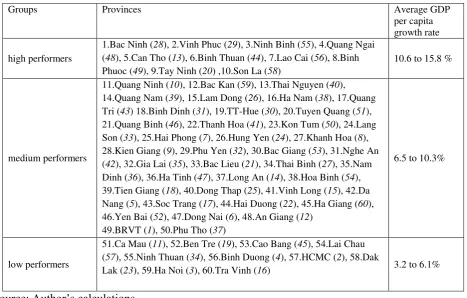
[image:5.595.64.532.414.712.2]In order to transform its centrally planned economy towards a more market-oriented economy, the Vietnamese government declared a reform planned called doi moi in 1986. The reform plan included economic and political reforms to foster economic growth and improve welfare of its residents. The doi moi reforms made a great contribution to the improvement of life standards in Vietnam. Real GDP per capita in Vietnam grew around 5.5% between 1990 and 2015 on average, rising from 8.3 to 31.4 million of Vietnamese Dong (in 2010 VND) (World Development Indicators, 2016). As a result of fast economic development, Vietnam transformed into a lower middle-income country from one of the poorest countries in the world. Welfare increase at province level, however, was uneven, some provinces performing much better than others in raising life standards. Table 1 below presents the performance of 60 provinces in GDP per capita growth from 1999 to 2010. Table 1 ranks GDP per capita growth performance of provinces from highest to lowest in terms of growth rate, while the ranking of provincial GDP per capita in 1999 is given in parenthesis next to provinces. Prior to 1999, there were several adjustments (splitting and re-establishing of provinces) in provincial administrative boundaries. For instance, from five provinces emerged ten provinces in 1996 and eight new provinces came into existence in 1997. Such adjustments resulted in irregularity in GDP per capita data even in the following year. Therefore, we start the period from 1999 to the last available data point, 2010. Furthermore, we excluded three new provinces, namely Dak Nong, Hau Giang and Dien Bien that were given province status in 2004 due to incomplete data for the period in question.
Table 1 Performance of province by real GDP per capita growth 1999-2010
Groups Provinces Average GDP
per capita growth rate
high performers
1.Bac Ninh (28), 2.Vinh Phuc (29), 3.Ninh Binh (55), 4.Quang Ngai
(48), 5.Can Tho (13), 6.Binh Thuan (44), 7.Lao Cai (56), 8.Binh
Phuoc (49), 9.Tay Ninh (20) ,10.Son La (58)
10.6 to 15.8 %
medium performers
11.Quang Ninh (10), 12.Bac Kan (59), 13.Thai Nguyen (40),
14.Quang Nam (39), 15.Lam Dong (26), 16.Ha Nam (38), 17.Quang
Tri (43) 18.Binh Dinh (31), 19.TT-Hue (30), 20.Tuyen Quang (51),
21.Quang Binh (46), 22.Thanh Hoa (41), 23.Kon Tum (50), 24.Lang
Son (33), 25.Hai Phong (7), 26.Hung Yen (24), 27.Khanh Hoa (8),
28.Kien Giang (9), 29.Phu Yen (32), 30.Bac Giang (53), 31.Nghe An
(42), 32.Gia Lai (35), 33.Bac Lieu (21), 34.Thai Binh (27), 35.Nam
Dinh (36), 36.Ha Tinh (47), 37.Long An (14), 38.Hoa Binh (54),
39.Tien Giang (18), 40.Dong Thap (25), 41.Vinh Long (15), 42.Da
Nang (5), 43.Soc Trang (17), 44.Hai Duong (22), 45.Ha Giang (60),
46.Yen Bai (52), 47.Dong Nai (6), 48.An Giang (12)
49.BRVT (1), 50.Phu Tho (37)
6.5 to 10.3%
low performers
51.Ca Mau (11), 52.Ben Tre (19), 53.Cao Bang (45), 54.Lai Chau
(57), 55.Ninh Thuan (34), 56.Binh Duong (4), 57.HCMC (2), 58.Dak
Lak (23), 59.Ha Noi (3), 60.Tra Vinh (16) 3.2 to 6.1%
Source: Author’s calculations.
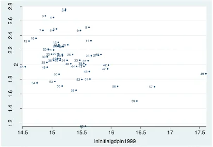
5 Real GDP per capita growth of the five provinces was higher than the median growth of 8.13% of 60 provinces from 1999 to 2010. As for low performers HCMC, Ha Noi and Binh Duong along with the least successful member of medium performers, BRVT, were four richest provinces in 1999. The disparity in growth rates between rich and poor provinces implies that poor provinces may have been catching-up with rich ones over the period. The fact that the ratio of real GDP per capita of the richest to that of the poorest decreased from 21.26 to 19.87 reinforces the view that the catching-up process took place from 1999 to 2010, albeit at low levels. In order to inspect the catching-up process visually, we plot per capita income growth rate of provinces from 1999 to 2010 against the “initial” (1999) level of per capita income in Figure 1 below. Instead of province names, the rankings of GDP per capita growth performance of provinces from 1999 to 2010 in Table 1 are presented in Figure 1. It is also visible in Figure 1 that Binh Duong (56), HCMC (57) and Ha Noi (59) with high level of initial GDP per capita scored low growth rates while Bac Ninh (1), Ninh Binh (3) and Bac Kan (12) with low level of initial GDP per capita scored high growth rates over the same period.
Figure 1 GDP per capita growth from 1999 to 2010 relative to initial level of GDP per capita in 1999.
Furthermore, as Table 1 and Figure 1 indicate that there is variation in economic growth among poor provinces. Although they all belonged to the ten poorest provinces club, Cao Bang and Lai Chau were outperformed by Ninh Binh, Lao Cai and Son La. Such discrepancy in growth rates can be attributed to the impact of geographic location on economic development.
1 2 3 4
5 6
7 8 9
10
11
12 13
14 15 16 17 1819 20 21
22
23 2429 26 28 2725 30 3132
33 34 35
36 37
38 40 39
41 42
43 44
45 46 47
48 49 50 51 52 53 54
55 56 57
58 59 60 1 .2 1 .4 1 .6 1 .8 2 2 .2 2 .4 2 .6 2 .8
14.5 15 15.5 16 16.5 17 17.5
6
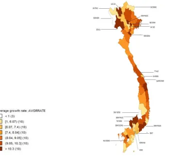
Figure 2 the average real GDP per capita distribution of provinces from 1999-2010
Sources: Author’s calculation. 3 areas without colour indicate excluded provinces of Dak Nong, Hau Giang and Dien Bien.
Provinces are divided into seven classes in terms of average growth rate, each class having ten provinces except the first one indicating 3 excluded provinces. Lightest colour presents the ten low performers as presented in Table 1. Two of them, Cao Bang and Lai Chau are in the north of the country. While rich provinces in the south such as BRVT, HCMC, Binh Duong and Dong Nai scored relatively low average growth rates below 7.4%, their neighbours Binh Thuan, Tay Ninh and Binh Phuoc grew around 11% over the same period. A similar pattern is seen in the north when we compare the growth rate of Ha Noi to that of its neighbours, Bac Ninh and Vinh Phuoc. Ranked third richest province in 1999, the growth rate of Ha Noi was below 6.1% while its two neighbours achieved a growth rate above 10.3%. Sixth richest province in 1999, Da Nang is also outperformed by its two neighbours TT-Hue and Quang Nam as we see in Figure 2. It seems that having rich neighbours can be a determinant of differences in income across provinces in Vietnam.
7
IV. Model and data
Based on a Solow growth model augmented with human and physical capital (Mankiw et al., 1992), our specification is in panel form (Islam, 1995) and can be stated as follows:
𝑙𝑛𝑦𝑖,𝑡= 𝛽0 𝑙𝑛𝑦𝑖,𝑡−𝑠 + 𝛽1 𝑙𝑛𝑠𝑘𝑖𝑡+ 𝛽2 𝑙𝑛𝑠ℎ𝑖𝑡+ 𝛽3 ln (𝑛𝑖𝑡+ 𝑔 + 𝛿) + 𝜇𝑖+ 𝜃𝑡+ 𝜀𝑖𝑡 (1)
where yitis the per capita real GDP (2005=100) in province i at time t. Both yitand explanatory
variables are averaged over four non-overlapping periods of 3 years from 1999-2010. lnyi,t-s denotes
the lagged dependent variable s years ago. skitand shit represent physical and human capital
investment, respectively. (nit + g+ ) is the sum of the average population growth rate over the
period, technological progress and a depreciation rate. In line with Mankiw et al. (1992), the sum of last two terms (g+ ) is assumed to be 0.05. The error term includes a time-constant province effect
i, a time-specific effect t and an idiosyncratic error term it. skit is measured as the ratio of
physical investment to GDP, while shit is proxied by pupils in high school per population. We
estimate the model with data on 60 provinces, yielding an unbalanced panel dataset with 238 observations due to incomplete data on population for two provinces1 Data are compiled from various sources published by the General Statistics of Vietnam (GSO). GDP, GDP per capita and physical investment data in (VND) come from Provincial Statistical Yearbook 1990-2010 by Provincial Statistics Office. The number of pupils in high school and population data are taken from Vietnam Statistical Yearbook 1985-2010.
Table 2 Descriptive Statistics
Variable Mean Median Standard Deviation Minimum Maximum
Real GDPpercapita 9899773 7201976 12330600 2471289 111622592
Lagged real GDP per capita 8450104 6104753 11666148 2080099 119640576
Physical capital investment 0.468 0.439 0.211 0.076 1.587
Human capital 0.106 0.107 0.021 0.048 0.163
Population growth+g+δ 0.061 0.057 0.025 0.003 0.384
Real GDP per capita is measured in VND. In Table 2, maximum value of GDP per capita warrants attention as it is more than 15 times of its median. Having petrol income separates BRVT from its peers with maximum GDP per capita value around 11.2 million of VND. Maximum GDP per capita value of BRVT is also reflected in lagged real GDP per capita. As far as physical capital investment is concerned, a Vietnamese province on average received physical capital investment equivalent of 46.8% of its GDP over the period. As for human capital, the mean value is 0.106 implying that on average around 10.6% percentage of population of a Vietnamese province were in high school from 1999 to 2010. In inspecting high values of population growth+g+δ in Table 1 we come across two
8 rich provinces, scoring 3rd and 4th richest in 1999, Ha Noi and Binh Duong, caused by immigration from other provinces.
V. Econometric methodology
Fingleton and López-Bazo (2006) and Lesage and Fischer (2008) draw attention to the problem of spatial dependence in growth regressions. This problem may arise due to pecuniary externalities from neighbouring regions (captured by spatial lag) or spatial autocorrelation among regression error terms (captured by spatial errors). If untreated, the presence of former leads to biased and inconsistent estimates because correlation between spatially lagged dependent variable and explanatory variables results in model producing parameter estimates larger or smaller than the true model whereas the presence of the latter leads to inefficient parameter estimates. To deal with spatial dependence between provinces, a spatially lagged dependent variable is added to equation 1 as follows:
𝑙𝑛𝑦𝑖,𝑡= 𝛽0 𝑙𝑛𝑦𝑖,𝑡−𝑠 + 𝛽1 𝑙𝑛𝑠𝑘𝑖,𝑡+ 𝛽2 𝑙𝑛𝑠ℎ𝑖,𝑡+ 𝛽3 ln (𝑛𝑖,𝑡+ 𝑔 + 𝛿) + 𝜌𝑊𝑙𝑛𝑦𝑗,𝑡+ 𝜇𝑖+ 𝜃𝑡+ 𝜀𝑖𝑡 (2)
where W is a row standardized weight matrix and ρ measures the strength of spatial dependence between provinces.
On the other hand, the spatial-error model can be stated as follows:
𝑙𝑛𝑦𝑖,𝑡= 𝛽0 𝑙𝑛𝑦𝑖,𝑡−𝑠 + 𝛽1 𝑙𝑛𝑠𝑘𝑖,𝑡+ 𝛽2 𝑙𝑛𝑠ℎ𝑖,𝑡+ 𝛽3 ln (𝑛𝑖,𝑡+ 𝑔 + 𝛿)+ 𝜇𝑖+ 𝜃𝑡+ 𝜔𝑖𝑡
𝜔𝑖𝑡 = 𝜆𝑊𝜀𝑖𝑡+ 𝑣𝑖𝑡 (3)
where the error term of province i depends on the error term of neighbouring provinces on the basis of weight matrix (𝑊𝜀𝑖𝑡) and an idiosyncratic component vit.
The structure of the weight matrix is usually unknown as the structure of spatial dependence between provinces is unknown a priori. Therefore, in the literature, various weight matrices have been used including nearest neighbours, contiguity, and distance cut-off matrix. The first two assume equal interaction between the sets of neighbouring geographic units, while the third type allows for interaction between any number of regions situated anywhere in the country. In the latter case, the extent of dependence falls and eventually becomes zero as the distance between geographical regions increases and reaches a maximum level.
9 province to interact with. This condition is satisfied at a maximum of 163 km. We test the robustness of our results by increasing the maximum distance first to 200 km (with a minimum of 3 ‘neighbouring’ provinces) and then to 300 km (with a minimum of 7 ‘neighbouring’ provinces).
In estimating models 2 or 3, we are likely to face endogeneity problem for two reasons. First, adding a spatially-lagged dependent variable (𝜌𝑊𝑙𝑛𝑦𝑗,𝑡) in model 2 causes a simultaneity problem. Secondly, there might be two-way causality between provincial GDP per capita and the right hand side variables in equation 1, leading to correlation between the explanatory variables and the error term. For example, physical capital is a determinant of economic growth but the latter is also likely to ensure easier access to capital for investment in fast-growing provinces. Similarly, fast-growing provinces can potentially create conditions conducive to population growth, causing two-way causality between economic growth and population growth. Two-way causality is also likely to be the case with respect to human capital as income growth provides better incentives as well as greater opportunities for investment in human capital (Bils and Klenow, 2000). Finally, the lagged real GDP per capita in equation 2 is also endogenous because it is correlated with the error term.
These sources of reverse causality and endogeneity can be addressed through a general method of moments (GMM), which corrects for both simultaneity/reverse causality and endogeneity problems (Madariaga and Poncet ,2007). Therefore, we adopt a GMM estimator (Arellano and Bond, 1991; Arellano and Bover, 1995; Blundell and Bond, 1998), which estimates a system of two equations with instrumented endogenous variables: - one in levels and the other in first differences. The instruments consist of differenced explanatory variables and lagged values of differenced explanatory variables, respectively. The number and validity of instruments along with the absence of second order autocorrelation in residuals warrant attention whilst using system GMM. As a rule of thumb, we keep the number of instruments below the number of provinces lest many instruments fail to purge endogeneity (Roodman, 2006). We use Hansen and Arellono Bond (AB) tests for the validity of instruments and the absence of second order-correlation, respectively. As it is more efficient than one step, we opt for two step variant of GMM with Windmeijer (2005) finite sample correction to address the downward bias in small samples. Finally, we conduct Lagrange Multiplier (LM) and robust LM tests to verify whether a spatial-lag (model 2) or spatial-error model 3) specification is more appropriate.
VI. Results
10
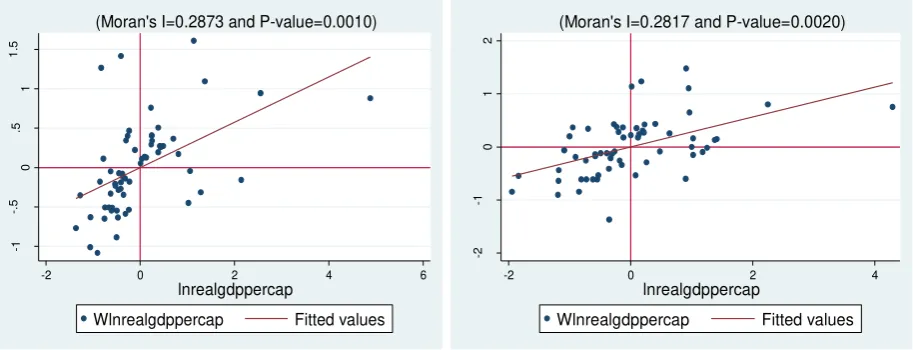
Figure 3: Moran scatter plots
A. First period (1999-2001) B. Fourth period (2008-2010)
The Moran’s I values of 0.2873 and 0.2817 along with p values for GDP per capita of Vietnamese provinces imply the existence of low to medium positive spatial autocorrelation. The null hypothesis that there is no autocorrelation is rejected at 1% significance for both periods. Visual inspection of Figure 3A and 3B also reveals the existence of positive autocorrelation. The majority of corresponding spatially lagged values of GDP per capita to those of provinces fall into high-high (upper right) and low-low (lower left) quadrants, implying positive spatial auto-correlation.
We present estimation results in Table 3. At the bottom of the table, we present diagnostic tests and information associated with the estimations. We test whether the spatial lag or the spatial error model is more appropriate using the Lagrange Multiplier (LM) and the robust LM tests proposed by Anselin (1988). According to the robust LM test, the hypothesis of no spatial error model is not rejected at 10% while the hypothesis of no spatially lagged variable is clearly rejected at 1%. Therefore, we consider only the spatial lag model in our estimations. Taken the absence of second order correlation confirmed by Arellano and Bond (AB) test together with the Hansen test result, we conclude that the lagged variables are valid instruments.
In columns 1 – 7 of Table 3, we report results from different estimators for comparison. We do not report fixed-effect estimation results to save space and because the F-Test for the absence of province-specific fixed effects does not reject the null hypothesis that all province-province-specific fixed effects are zero. Estimated coefficient on the lagged per capita GDP (β0) indicates convergence among
provinces’ per-capita GDP if it is less than 1 but divergence if it is greater than 1.
-1
-.
5
0
.5
1
1
.5
-2 0 2 4 6
lnrealgdppercap
Wlnrealgdppercap Fitted values
(Moran's I=0.2873 and P-value=0.0010)
-2
-1
0
1
2
-2 0 2 4
lnrealgdppercap
Wlnrealgdppercap Fitted values
11 Table 3: Baseline results (with cut-off distance of 163km, minimum of 2 neighbouring province)
Pooled OLS Between effects ML System GMM
(1) (2) (3) (4) (5) (6) (7) (8) (9)
Lagged GDP per capita 0.996*** (0.008) 0.991*** (0.009) 1.012*** (0.013) 1.008*** (0.014) 0.992*** (0.014) 0.990*** (0.145) 1.003*** (0.017) 0.967*** (0.023) 0.970*** (0.018) Physical capital investment 0.032** (0.014) 0.034** (0.014) 0.047** (0.018) 0.050*** (0.018) 0.036*** (0.014) 0.024 (0.015) 0.115*** (0.043) 0.128** (0.062) 0.088*** (0.07) Human
capital 0.033 (0.028) 0.038 (0.031) 0.054 (0.038) 0.060 (0.039) 0.103*** (0.032) 0.065** (0.032) 0.097* (0.056) 0.130* (0.081) 0.080* (0.049)
Population
growth+g+δ -0.019* (0.011) -0.020* (0.011) -0.020 (0.034) -0.022 (0.034) -0.008 (0.017) -0.004 (0.017) -0.030* (0.018) -0.038** (0.019) -0.028** (0.015) Spatially
lagged GDP per capita
0.020
(0.021) 0.017 (0.022) 0.067*** (0.020) 0.027 (0.023) 0.147* (0.079) 0.070** (0.035)
Constant 0.225**
(0.106) -0.011 (0.272) 0.131 (0.300) -0.078 (0.402) -0.555** (0.249) 0.308 (0.313) -1.338 (0.925) -0.335 (0.438)
R-squared 0.98 0.98 0.99 0.99 0.97 0.97
Time
Dummies Yes Yes Yes Yes No Yes Yes Yes Yes
F test for all
i=0a
(p-value)
0.14 0.15
AB test for
AR(2)b
(p-value)
0.208 0.680 0.332
Hansen test c
(p-value) 0.514 0.734 0.651
Number of
Instruments 39 42 42
Implied convergence
rate % (λ)d
0.13 0.30 -0.40 -0.27 0.27 0.34 -0.10 1.12 1.02
Spatial Error LM/Robust
LM 5.1** (0.03) / 2.6 (0.11)
Spatial Lag LM/Robust LM
11.1*** (0.00) / 8.6*** (0.00)
Notes:Stata is used to conduct the estimations. Standard errors are in parentheses. ***, **, * indicate significance at the 10%, 5%, 1% level. We limit the maximal lag length to 2. Both the LM and Robust LM tests follow a chi-squared distribution with one degree of freedom and p-values are presented in parentheses.
a The null hypothesis that all province related fixed effects are zero.
bThe null hypothesis is that there is no second-order autocorrelation in the errors of the first-differenced
equation.
c The null hypothesis is that there is no correlation between over-identifying instruments and the errors.
12 Combined with robust LM tests that favour the spatial-lag specification and the usual tests justify the use of system GMM. They indicate that failure to account for pecuniary externalities is highly likely to introduce omitted variable bias. Also, they indicate that failure to take account of endogeneity is likely to produce inconsistent parameter estimates. Results from the preferred specification (GMM with spatial lag) are presented in column 8 and 9 of Table 3. Results in column 8 indicate the existence of spatial dependence between income growth across Vietnamese provinces as the coefficient on the spatially-lagged income is positive and significant. Furthermore, we check whether our results are sensitive to exclusion of outliers. We winsorize the dependent variable (RealGDPpercap) at the 99th percentile (79 million of VND) and exclude three values exceeding the threshold. We report the results in column 9 in Table 3.2 After we exclude three outliers, we observe small decreases in the coefficients on physical capital investment, human capital and a very small increase in the coefficient on lagged GDP per capita while the coefficient on spatially-lagged GDP per capita halved. After removing the outliers, we obtain the preferred results in column 9.
The positive and significant coefficient on the spatially-lagged GDP per capita implies that a province benefits from income growth in neighbouring provinces. In other words, income per capita in a given province is positively associated with income in surrounding provinces. Lagged GDP per capita is significant at the 1% level across all columns in Table 3. The coefficient on lagged GDP per capita is greater than one in columns 3, 4 and 7 and indicates divergence; whereas it is less than one in columns 1, 2,5,6,8 and 9 and indicates convergence. The speed of convergence in column 9 after we control for spatial interdependence in income and remove outliers suggests that only about 1.02% of the gap between the initial equilibrium and the new equilibrium is eliminated per year.
As the Solow model predicts, physical investment is positively associated with higher GDP per capita growth. The coefficient for physical investment is significant at the 1% level in all the columns in Table 3. However, after the endogeneity issue is treated by system GMM, the coefficient on physical investment increased from a band 0.02 - 0.05 band to 0.09 in column 9. This finding suggests that higher levels of physical investment are associated with higher levels of income in the provinces. The result is similar for human capital as human capital has a positive impact on economic growth. In line with predictions of the augmented Solow model, population growth and depreciation rate tend to decrease per-capita income growth as the coefficient is negative and statistically significant at the 5% level in column 9.
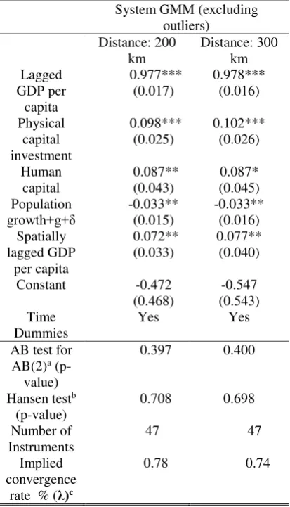
We check the robustness of our baseline results in column 9 of Table 3 to using higher thresholds in constructing the distance matrix. Initially, we increase the threshold to 200 km (with a minimum 3 neighbouring provinces) and then to 300 km (with a minimum of 7 neighbouring provinces). The results in Table 4 are in line with the baseline results in that they
2 In order to double-check, we use Cook’s distance (1982) to detect outliers. Cook’s distance measures the
13 confirm the presence of convergence and that of spatial dependence due to pecuniary externalities. When the distance cut-off is higher, the extent of spatial dependence is slightly greater while the rate of convergence is smaller.
Table 4. Robustness checks with different cut-off distance
System GMM (excluding outliers)
Distance: 200
km Distance: 300 km Lagged
GDP per capita
0.977***
(0.017) 0.978*** (0.016)
Physical capital investment 0.098*** (0.025) 0.102*** (0.026) Human capital 0.087** (0.043) 0.087* (0.045) Population
growth+g+δ -0.033** (0.015) -0.033** (0.016) Spatially
lagged GDP per capita
0.072**
(0.033) 0.077** (0.040)
Constant -0.472
(0.468) (0.543) -0.547 Time
Dummies
Yes Yes
AB test for AB(2)a
(p-value)
0.397 0.400
Hansen testb
(p-value) 0.708 0.698
Number of
Instruments 47 47
Implied convergence
rate % (λ)c
0.78 0.74
Notes:Stata is used to conduct the estimations. Standard errors are in parentheses. ***, **, * indicate significance at the 10%, 5%, 1% level.
a The null hypothesis is that there is no second-order autocorrelation in the errors of the first-differenced
equation.
b The null hypothesis is that there is no correlation between over-identifying instruments and the errors. c λ=-ln(𝛽
0)/s
VII. Conclusions
Our analysis suggests that failure to control for spatial dependence amounts to omitted variable bias and implies lack of convergence even though the latter exists. Taking account of endogeneity and spatial dependence, we find that economic growth in a province is positively associated with economic growth in surrounding provinces; and that the speed of convergences ranges from 0.74 to 1.02 per annum, depending on maximum distance between neighbouring provinces.
14 spatial dependence between provincial per-capita income growth increases from 0.070 to 0.077 as the distance between provinces increases from 163 km to 300 km. Similarly, the rate of convergence decreases from 1.02% to 0.74% over the same distance range. Beyond these main findings, we also report that the effects of human and physical capital on growth is positive and in line with findings in the wider literature. Therefore, we argue for inclusion of spatial dependence in regional/provincial growth estimations on theoretical grounds to take account of spatial externalities and on empirical grounds to avoid the risk of omitted variable bias.
Our findings have important policy implications in that they point out the risk of divergence between poor provinces surrounded by poor provinces in the north and medium or strong performers surrounded by strong performer in the middle or south of the country. Hence, there is a case for active regional policy that involves higher levels of investment in human and physical capital in Northern provinces in order to help them catch-up. These policy options can be combined with infrastructure and transport investment that strengthens the links between the poor provinces with more dynamic markets in the rest of Vietnam.
The limitation of studies estimating the impact of spatial spill-overs, including this study, is the inexistence of a method that identifies a unique weight matrix reflecting the connectivity between locations. Such a limitation makes it difficult to compare studies on regional economic growth across countries. The other limitation is related to data issues. Due to changes in administrative borders of provinces, our data set included only 60 provinces.
Future studies should incorporate institutional determinants into growth models at province level such as corruption, rule of law and red tape once data on these determinants are available for sufficiently long time periods to obtain reliable estimates.
References:
Abreu, M., de Groot, H. L. F. & Florax, R. J. G. M. (2004) Space and Growth: a Survey of Empirical Evidence and Methods, Tinbergen Institute Working Paper No. TI 04-129/3. Internet site: http://ssrn.com/abstract_631007
Anselin, L. 1988. Spatial Econometrics, Methods and Models. Dordrecht: Kluwer Academic Publishers.
Anwar S. and L. P Nguyen. 2010. “Foreign direct investment and economic growth.” Asia Pacific Business Review, 16(1-2): 183-202.
15 Arellano, M. and O. Bover. 1995. “Another look at the instrumental-variable estimation of error-component models”, Journal of Econometrics, 68, 29–52.
Bai, C-E., MA H., Pan W. 2012. “Spatial spillover and regional economic growth in China.”
China Economic Review, doi:10.1016/j.chieco.2012.04.016
Bils, M.; Klenow, P. J. 2000. “Does schooling cause growth?”,American Economic Review, 90, (5), 1160-1183.
Blundell, R. and S. Bond. 1998. “Initial conditions and moment restrictions in dynamic panel data models”, Journal of Econometrics, 87, 115–43.
Cook, R. Dennis; Weisberg, Sanford (1982). Residuals and Influence in Regression. New York, NY: Chapman & Hall.
Cravo, A. C., Becker B., Gourlay, A. 2015. Regional Growth and SMEs in Brazil: A Spatial Panel Approach. Regional Studies, 49(12), 1995-2016.
Cuaresma, J. Crespo., Doppelhofer G., & Feldkircher M. 2014. “The Determinants of Economic Growth in European Regions”, Regional Studies, 48(1), 44-67.
Ertur, C., Le Gallo, J., & Baumont, C. (2006). “The European regional convergence process,
1980-1995: Do spatial regimes and spatial dependence matter?”.International Regional Science Review, 29(1), 3-34.
Fingleton, B. and E. López‐Bazo. 2006. “Empirical growth models with spatial effects.”Papers
in Regional Science, 85(2), 177-198.
Fujita M, Krugman P and Venables A (1999) The Spatial Economy: Cities, Regions, and
international Trade. MIT Press, Cambridge, MA.
Islam, N. 1995. “Growth empirics: a panel data approach.”The Quarterly Journal of Economics, 110(4): 1127-1170.
Le Gallo J. 2004. Space-time analysis of GDP disparities among European regions: A Markov chains approach. International Regional Science Review 27: 138-65.
LeSage J. P. and M.F. Fischer. 2008. “Spatial growth regressions: Model specification, estimation and interpretation.” Spatial Economic Analysis, 3(3): 275-304.
Lima, R, C. A. and Neto R.M.S. 2016. “Physical and Human Capital and Brazilian Regional Growth: A Spatial Econometric Approach for the Period 1970–2010.” Regional Studies, 50 (10): 1688-1701.
Madariaga N., and S. Poncet. 2007. “FDI in Chinese cities: Spillovers and impact on growth.” The World Economy, 30(5): 837-862.
16 Mohl, P. and Hagen T. 2010. “Do EU structural funds promote regional growth? New evidence from various panel data approaches”, Regional Science and Urban Economics, 40(5): 353-365. Resende G. M., de Carvalho A. X. Y., Sakowski P.A.M., Cravo T. A. 2016. “Evaluating multiple spatial dimensions of economic growth in Brazil using spatial panel data models.” The Annals of Regional Science, 56(1): 1-31.
Roodman D. 2009. “How to do xtabond2: An introduction to difference and system GMM in Stata.” The Stata Journal, 9(1): 86-136.
Tian, L., Wang, H., & Chen, Y. (2010). “Spatial externalities in China regional economic growth.”China Economic Review, 21, S20–S31.
The World Bank. 2015.”Transport in Vietnam.” Accessed January 20 2015
http://web.worldbank.org/WBSITE/EXTERNAL/COUNTRIES/EASTASIAPACIFICEXT/E XTEAPREGTOPTRANSPORT/0,,contentMDK:20458737~menuPK:2069374~pagePK:3400
4173~piPK:34003707~theSitePK:574066,00.html#Roads_and_Highways.
Torres-Preciado, V.H., Polanco-Gaytán, M. & Tinoco-Zermeño, M.Á. 2014. “Technological innovation and regional economic growth in Mexico: a spatial perspective” The Annals of Regional Science, 52(1): 183-200.
Windmeijer, F. 2005. “A finite sample correction for the variance of linear efficient two-step GMM estimators.” Journal of Econometrics,126: 25-51.
Notes on Contributors
Bulent Esiyok is an assistant professor in the Department of Economics, Baskent University, Turkey. His research interests include international trade, foreign direct investment, economic growth and competition.