Munich Personal RePEc Archive
What account for the differences in
rent-price ratio and turnover rate? A
search-and-matching approach
Huang, Daisy J. and Leung, Charles Ka Yui and Tse,
Chung-Yi
Nanjing Audit University, City University of Hong Kong, University
of Hong Kong
2017
Title:
What
account
for
the
differences
in
rent
‐
price
ratio
and
turnover
rate?
A
search
‐
and
‐
matching
approach
Author: Daisy J. Huang, Charles Ka Yui Leung and Chung‐Yi Tse
This version: February, 2017 Abstract
We build an on‐the‐house‐search model and show analytically that the rent‐to‐price ratio (or rental yield) and turnover rate, which are frequently used metrics for the housing market, are jointly determined in equilibrium. We therefore adopt a simultaneous equation approach on matched sale‐ rental pairs in our empirical investigation, as a housing unit cannot be owner‐occupied and renter‐ occupied at the same time. Our empirical results confirm a higher turnover rate is associated with a lower rent‐to‐price ratio, as predicted by the model. Furthermore, our results suggest a form of
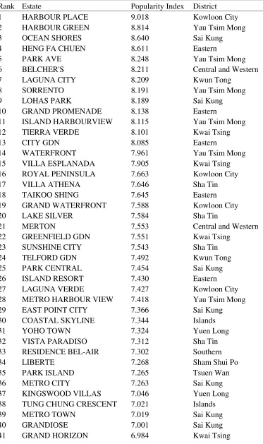
“dichotomy” in the empirical determinants of rental yield and turnover at the real‐estate‐development (RED) level: the demographic structure, and past return performance affect its turnover rate, while popularity, human capital environment, mortgage burden, and long run rent growth determine the rental yield. No evidence of “thick market effect” is found. The robustness of our results are established through a series of tests. In addition to these findings, our tractable search‐theoretic model, a ranking of more than 130 RED in Hong Kong based on the popularity index we construct, and the estimated brand‐ premium for different major real estate developers may also carry independent research and practical interests.
Keywords: housing rental yield, turnover rate, bootstrap, leave‐one‐out cross validation (LOOCV), matching estimator, 3 stages least squares (3SLS)
JEL Classification Numbers: D10, G10, R21
Acknowledgement: We are grateful to Been‐Lon Chen, Nan‐Kuang Chen, Man Cho, Gangzhi Fan, Shihe Fu, Richard Green, Cheuk Yin Ho, Mingming Jiang, Kamhon Kan, Yuichiro Kawaguchi, Shian‐Yu Liao, Steve Malpezzi, Masao Ogaki, Tim Riddiough, Jay Sa‐Aadu, Jim Shilling, Jingjing Tang, Wei Xiao, Haijian Zeng, seminar participants at the Asia‐Pacific Real Estate Research Symposium (2015, Cheng Du), Global Real Estate Submit (2015, Washington, D.C.), Taiwan Economic Association meeting (2016, Taipei), City University of Hong Kong, Guangxi University, anonymous referees for helpful comments. Financial support from the City University of Hong Kong and University of Hong Kong are gratefully
acknowledged. Part of this research is conducted when Leung is a visiting scholar of ISER, Osaka University, whose hospitality is gratefully acknowledged. Tommy Chan provides capable research assistance. The usual disclaimer applies.
1
Introduction
Rent-to-price ratio and turnover are both key elements in discussions of the housing market. One example is how the rent-to-price ratio, also known as the (gross) rental yield, is often used in the media and in the academic literature as a metric of the
pos-sibility that a “bubble” has formed.1 Similarly, turnover, also known as the trading or
transaction volume, is a commonly used metric for the “status” of the housing
mar-ket.2 However, theequilibrium determination of rent-to-price ratio is under-explored
in empirical works and policy discussion, making it difficult to assess whether the
observed rent-to-price ratio and turnover rate are “reasonable.” To put it differently,
what levels of the rent-to-price ratio and turnover rate are more likely to be
associ-ated with housing market mispricing?3 This study uses a straightforward method to
answer this question. First, we propose a simple equilibrium search-theoretic model, in which the rent-to-price ratio and the turnover rate are endogenously determined. 1Examples of using rent-to-price ratio as a measurement of the housing market abound in the media. For instance, in a widely used website, Global Property Guide (2010) states that “In the stock market a very popular rule of thumb involves the price-earnings ratio, which measures how high the company’s net earnings are, in relation to the price of the stock. . . . It’s the same in the housing market. What’s generally viewed as reasonable is similar to what’s considered reasonable in the stock market, although houses tend to be expected to yield slightly less, perhaps because a house’s value depreciates less over time than the assets of a typical company. The price/rent ratio (or gross rental yield) is the housing parallel to the price/earnings ratio.” (Italic added).
The rent-to-price ratio is also widely used in the academic literature. For example, in their investigation of possible mis-pricing of housing markets in China, Wu et al. (2012, p.533) states that “. . . The data show that price-to-rent ratios not only are high in these places, but they have increased sharply in the past few years. The price-to-rent ratio in Beijing increased by almost three-quarters just in the last three years, rising from 26.4 in 2007(1) to 45.9 in 2010(1). Hangzhou, Shanghai, and Shenzhen also have seen theirprice-to-rent ratios rise sharply to over 40. . . . Given what we think are reasonable assumptions about the other parameters determining user costs, it appears that home buyers are assuming quite large capital gains on their homes. . . . However, home prices do not always rise and certainly not consistently at the high rates recently experienced in China. . . one can conclude that house prices in major Chinese markets are quite risky, even though the data are too limited to make a blanket claim of mis-pricing.” (Italic added). Similarly, in a research report by the staff of the Reserve Bank of Australia, Fox and Tulip (2014) also use a constant-quality measure of rental yield to measure the degree of over-valuation.
More recently, Green (2015) acknowledges that in the evaluation of whether a “bubble” exists or not, it is not enough to consider the price only; the rent should also be taken into consideration.
2For example, Financial Times (2015) reports that as the global transaction volume of commercial real estate hits a record in the last quarter of 2014, “fear of bubble” arises among analysts. Similar statements can be found in the academic literature as well. For example, in their survey of different classes of “bubble models”, Brunnermeier and Oehmke (2013) write that “. . . heterogeneous-belief models generate the prediction that bubbles are associated with hightrading volume, something that is often observed in practice.. . . ” (Italic added). In the book coauthored by S. Gjerstad and Nobel laureate Vermon Smith (2014, p.21), it is written that “. . . before an asset bubble collapses,trading volume typically declines substantially. This occurred in the housing market. . . ” (Italic added).
We find, unsurprisingly, that the two variables are jointly determined at the equi-librium. This motivates us to take a simultaneous equations approach to identify the empirical determinants of both the rent-to-price ratio and turnover rate, taking into considerations that the two variables would interact in equilibrium. Our em-pirical framework can hence provide a benchmark for an estimate of “reasonable” rent-to-price ratio and turnover rate given the empirical determinants, which in turn constitute a yardstick for potential housing market mispricing. The details will be provided in later sections.
The search-theoretic approach to the study of real estate markets and urban economic issues has recently been the subject of much research (for example, Anglin, 2006; Anglin and Gao, 2011; Albrecht et al., 2007; Diaz and Jerez, 2013; Fisher et al., 2003; Genesove and Han, 2012; Krainer, 2001; Novy-Marx, 2009; Piazzesi and Schneider, 2009; Tse, 2011; Wheaton, 1990; Yavas, 1992a, 1992b). Many studies have examined equilibrium transaction price and trading volume, but the rental segment
of the residential real estate market appears to be under-explored.4 We take an initial
step in this regard by developing a search and matching model that enables landlords to choose whether to sell or to rent their properties. Thus, the equilibrium rental yield and the turnover can then be derived endogenously. Changes in real estate development (RED) level variables are demonstrated to induce a negative correlation between rental yield and normed transaction. Our simple framework is tractable and can be further extended for other research projects. Hence, it may carry independent research interest.
Our second contribution is to propose a simultaneous equations system to account for endogenously correlated rental yield and turnover rate, instead of the usual
or-dinary least squares estimation.5 We employ the Hong Kong data for our empirical
testing based on the following reasons. First, Hong Kong provides a housing market in which the owner-occupied and rental segments are “integrated,” in the sense that the same unit can be used for both types of housing. Owners can hence arbitrage
for different opportunities and so the rent-to-price ratio is maintained at a level that
reflects a “no-arbitrage” situation. The population density of Hong Kong is high and
most people live in units in high-rise condominiums, which are for sale and for rental.6
In contrast, the for-sale housing in the United States is typically detached houses, while rental housing is concentrated in the apartment buildings, many of which are owned by institutional investors. Thus, the two housing markets are virtually segre-gated, hence limiting the arbitrage opportunities for individual house owners. The
standard rent-to-price ratio may therefore not be as informative (Glaeser and
Gy-4Xiao (2014), Sato and Xiao (2015) explore the relationship between house rent and labor market. Their models do not have housing price though.
5More specifically, we implement three-stage least squares estimation on a two equation system with rental yield and turnover rate treated as endogenous variables and on the same footing.
ourko, 2007, Malpezzi, 2014, among others). We have access to RED level data in
Hong Kong, which helps us to mitigate the potential aggregation bias.7 More
specif-ically, our sample covers 130 major private REDs in Hong Kong during the period from November 2011 to October 2012. This choice of sampling period enables us to include corresponding information about demographics, household income, and
hous-ing related expenditure from the official census.8 The rent-to-price ratio and normed
transactions are constructed out of the micro-transaction data. We also construct a “popularity” index based on a formative measurement model, and attempt to make
it as composite as possible.9 This index may therefore independently be of interest
for academic research and practical business investment.
In addition to constructing the popularity index, we have several other majorfi
nd-ings. First, our three-stage least squares (3SLS) estimation confirms our theoretical
model and suggests significantly negative effects of turnover and popularity on the
rent-price ratio. If the normalized transaction increases by one standard deviation,
other things being equal, the associated rental yield would be048standard deviations
lower. If the popularity index increases by one standard deviation, its rent-to-price
ratio would be lower by almost016standard deviations, holding other variables
con-stant. On the other hand, neither the estimate coefficient of the popularity index
nor that of the rent-to-price ratio of the RED, is statistically significant in explaining
the turnover rate.10 Second, weidentify some (potential) empirical determinants of
the rent-to-price ratio and the turnover rate, controlling for the popularity index and the endogenous variables. As a demand shifter, increases in income should stimulate sales volume, but a higher income also means a higher opportunity cost of moving.
Ex ante, it is not clear which will be the dominant force, but our empirical finding
suggests it will be the latter. Third, we identify a form of empirical “dichotomy”
in the housing market. The demographic structure, and past return performance of
a real estate development tend to affect its turnover rate, while popularity, human
capital environment, mortgage burden, and long-run rent growth have more influence
on rental yield. Last, we obtain direct evidence on the brand value ranking of nine
main developers in Hong Kong residential property development market. We also
find occupational exposure to real estate has significant and positive impacts on the
valuation ratio of rental yield, but not on trading intensity, which is consistent with
the confirmed moral hazard effect in real estate brokerage.11
7See Hanushek et al. (1996) for more discussion, among others.
8The Census and Statistics Department of the Hong Kong government has published, thefirst time in Hong Kong history, RED level statistics for free public access after the 2011 Census.
9It takes into account all factors that are accessible to us and potentially relevant in housing purchase decision, such as affordability, location appeal, access to public transportation, developer reputation, architectural design, surrounding environment, school zone, building age, facility, etc.
10On the other hand, we do identify other variables that are significant in explaining the RED level turnover rate. Please see below.
Our paper can also be broadly considered as a study of the asset market
liq-uidity (e.g. Amihud et al. 2013), as real estate is an asset traded with significant
frictions. There are recent studies of the rent-to-price ratio that also use a search-theoretic framework. For instance, Kashiwagi (2014) considers a search search-theoretic model with two sub-markets (“locations”). Homeowners in a location receiving “sep-aration shocks” are forced to sell their houses immediately, move to another location and become renters in the next period. Renters who do not receive separation shocks would attempt to purchase a house. In that sense, Kashiwagi’s model may be closer
to the inter-regional mobility discussed in the literature, i.e. a situation when
eco-nomic agents are relocated among different states or cities that are far from each
other. Hence, it is natural for Kashiwagi (2014) to calibrate his model to match the aggregate data of the US. In terms of modelling strategy, the assumption that homeowners need to sell their houses immediately and move to another location is analogous to the “job destruction model” developed in the seminal work of Mortensen
and Pissarides (1994), where workers need to search for new jobs once they receive
the separation shocks, because their jobs are “destroyed.” Kashiwage also proves the existence and uniqueness of a symmetric steady state. Our model instead assumes
that mismatched households can stay in their original homes until they find new
ones, as houses are not “destroyed” after the separation shocks. It may therefore
be applicable to the situation ofintra-regional mobility orintra-metropolitan mobility
discussed in the literature, which is also consistent with our empirical implementation
of using micro-data from a single city.12 In terms of modelling strategy, as agents in
our model are allowed to stay in the houses even after receiving separation shock, our model has some parallel to the “on-the-job search” model in the labor market search
literature. In those models, workers who are not satisfied with the current job-wage
package would nevertheless stay in the current jobs until they find “better ones”
(Burdett and Mortensen, 1998; Pissarides 1994). We also prove that a unique steady state exists in that environment. Halket and Pignatti (2013) also study the rent-to-price ratio in a search-theoretic housing market model. Their focus is whether rental housing is available in the local market and how the rent-to-price ratio will relate to the homeownership rate in equilibrium. They do not elaborate the relationship between the rent-to-price ratio and trading volume, which is one of the focuses of this paper. They also propose a competitive search model (CSM) while we adopt a
random search model (RSM),13 and it is well known that CSM and RSM can deliver
very different conclusions on similar issues.14 The data sets in these previous studies
12The literature on intra-regional or intra-metropolitan mobility has a long history. Among others, see Quigley and Weinberg (1977) for a review of the earlier literature, and Zax (1994) for a recent analysis. See also Green and Malpezzi (2003).
13For another example of CSM in real estate, see Leung and Zhang (2011), among others. 14For instance, see Moen and Rosen (2004), and the reference therein.
are from the United States, while ours is from an Asian city, and we adopt a 3SLS estimation methodology. Our work should therefore be considered complementary to that in these other studies.
Recently, the liquidity of the housing market is studied empirically. For instance, Kwok and Tse (2006) investigate the price premia for easy-to-sell condominiums in
one administrative district of Hong Kong in 2005. Using data from 24 major office
markets in the U.S. from 1995 to 2010, Liu and Qian (2012)find a bust period driven
illiquidity premium in the real estate expected returns. We complement these studies by adopting the simultaneous equations approach and by combining housing market
data with household data (in this case, the 2011 Census of Hong Kong). The trade-off
is that we are unable to examine the time series variations of the rent-to-price ratio, as the 2011 Census is a cross-sectional survey by nature. We leave this to future research.
Ourfindings are also connected to the literature on real estate capitalization rates,
which focuses on four categories of cap rate determinants: macroeconomy (Ambrose and Nourse 1993; Evans 1990; Jud and Winkler 1995), property attributes (Peng 2013), investor characteristics, as well as regional market conditions including ex-pected returns and rent growth rate (An and Deng 2009; Campbell et al., 2009; Plazzi et al., 2010), vacancy rate (Sivitanidou and Sivitanides 1999), investor sen-timent (Clayton et al., 2009), and credit availability (Chervachidze and Wheaton 2013). We demonstrate in the context of the Hong Kong market that the property’s physical attractiveness, earnings potential, and household characteristics all matter in the determination of housing rent to price ratio. However, short-term housing price
appreciation rate does not seem to be significant.
The organization of the remainder of this paper is straightforward. The next sec-tion presents a simple theoretical model. We then describe our empirical methodology, which is followed by a discussion of the data. Empirical results are then presented, and the concluding remarks are given in the last section.
2
Theoretical Analysis
2.1
Model setup
2.1.1 Basic Environment
In our theoretical model, time runs continuously from zero to infinity. The population
of households is normalized to unity, of which a fractiondemand to reside in for-sale
housing and the remaining fraction (1−) demand rental housing.15 The housing
stock is exogenously given at some value assumed to exceed the population of
households at unity, each unit of which can be used for either for-sale or rental
housing.16
A household in either for-sale or rental housing who finds their current dwelling
suited to their needs is referred to as a matched household as opposed to a mismatched household — one who desires to move because the current dwelling no longer meets the household’s needs. We model the distinction between matched and mismatched
households by assuming that the former, but not the latter, receive a flow utility
0 per time unit. Matched households are subjected to periodic moving shocks,
after which they become mismatched with their current dwellings. The shocks are meant to model events such as job relocation, separation, the loss of family members, etc., that necessitate the need to change housing. Because such shocks typically occur independent of the state of the housing market, it is natural to treat them as exogenous to the market. Formally, we model the occurrence of the shocks as
Poisson processes with an arrival rate equal to some value we denote as 17 An
intuitive interpretation is that a given household would be hit by a moving shock at
an instantaneous probability over each unit of time.
When an owner-occupier is mismatched, the household remains in the old house while searching for a new house to buy. The household vacates the old house once the
household finds a new house to move into, but not before.18 Similarly, when a rental
household is mismatched, the household remains in the old house while searching for a new house to rent. Once a new house is found, the household breaks the lease
and leaves the old house. An owner of a vacant house chooses between offering his
property for sale and for rent — whichever option offers the higher expected discounted
returns.
15In this paper, we assume that renters and owner-occupiers would not change their identities. This assumption has two major merits. First, Jovanovic and Rosenthal (1988) show that in an anonymous game (of which market equilibrium is a special case) where agents are not allowed to change their identities, the existence and certain properties of equilibrium are guaranteed. Second, endogenizing the tenure choice (i.e., rent or own) in a frictional housing market is by no means a simple problem. For a flavor of the complexity involved, see Chambers et al. (2009) which study households’ tenure choices, with price and rent endogenously determined, in a life-cycle model without search friction. We believe that the goal of the theoretical analysis in this paper — to construct the simplest model possible in which the transaction volume and the rent-to-price ratio are determined simultaneously in equilibrium — is better served with a model in which tenure choices are exogenously given.
16See also Leung and Tse (2016), in which the stock of owner-occupied houses is assumed to be less than the population of households demanding such housing whereby a fraction of those households must stay in rental housing temporarily at each moment in time.
17The assumption of exogenous separation shock is the “standard” assumption in the labor market search literature, which can be traced back to Mortensen and Pissarides (1994), among others.
2.1.2 Matching rate and Market Tightness
The model housing market is a decentralized market in which imperfectly informed buyers and sellers engage in time-consuming search for trading partners, the outcome of which, as in Pissarides (2000), is modeled by a matching function. In particular,
we assume that if there aree would-be buyers and vacant houses for sale, there
would be
³ e
´
bilateral meetings between pairs of buyers and sellers over a
unit of time, where( )is an increasing, concave, and constant returns function.19
For an individual buyer, a meeting with a seller comes about at the Poisson arrival
rate
³ e
´
e, whereas the arrival rate of meetings for an individual seller
is
³ e
´
. Now,
³ e ´ = ³
1 ´
, given that ( )
is constant returns to scale. Then, we can write the meeting rate for sellers as
()≡ ³
e
´
=(1), where ≡e denotes the ratio of
the measures of buyers to sellers, or what is known as the market tightness, in the
for-sale market. The meeting rate for buyers () ≡
³ e
´
e can be
shown to be equal to(). With the matching function increasing and concave
in both arguments,
()
0
2
() 2
0 ()
0
2
() 2
0 (1)
The upshot of all this is that the meeting rates for buyers and sellers are functions of the tightness of the market only, independent of the scale of the market due to the constant-returns assumption on the matching function. Intuitively, in a tighter
market as manifested by a larger , there are more buyers for each seller and as a
result, it would be easier for an individual seller to meet a potential buyer and the converse holds for an individual buyer.
A bilateral meeting does not guarantee that the house in question is a good match for the would-be buyer though. We assume that the would-be buyer indeed
finds the house a good match with probability ∈ (01).20 Then, the instantaneous
probability (Poisson arrival rate) at which a buyer finds a suitable house to buy is
19For instance, Blanchard and Diamond (1990) show that the aggregate matching function in the labor market in the U.S. is indeed subject to constant returns to scale. A few subsequent studies have substantiated the finding in various different contexts. See Petrongolo and Pissardes (2001), among others, for a review of the literature.
20Here we assume that the “match quality” is either 1 or 0, with respective probabilities and
(), whereas the instantaneous probability (Poisson arrival rate) at which a seller
successfully sells is ().
The same search and matching framework is imposed on the rental market.21
In particular, over a unit of time, there would be
³ e
´
bilateral meetings
between pairs of individuals from the two sides of the market, where ( ) is an
increasing, concave, and constant returns to scale matching function and e and
the respective measures of rental households who are on the market and owners
of for-rent vacant houses. Then, the instantaneous probability (Poisson arrival rate)
at which a landlord successfully finds a tenant is () and the instantaneous
probability (Poisson arrival rate) at which a rental household successfullyfinds a house
is (), where () ≡ (1), () = (), and = e
is the tightness of the rental market. Given the assumptions on ( ), we have,
analogous to()and()for the for-sale market,
()
0
2
() 2
0 ()
0
2
() 2
0 (2)
2.1.3 Expected Discounted Payoff, Price, and Market Rental
A key element of our model is how owners of vacant houses decide between offering
their properties for sale and for rent. To proceed, we first assume that all actors in
the housing market are risk neutral. Second, we should restrict attentions to studying steady-state equilibrium of the housing market in which the measures of households in various states are unchanging through time.
Consider first a matched household in an owner-occupied house. Over a unit
a time, the household enjoys the flow utility while staying in a matched house.
But then, the match can be broken at each moment in time at an instantaneous
probability , after which the given household becomes a mismatched household. A
forward-looking risk-neutral matched household then has expected discounted payoff
satisfying,
=+³f−´ (3)
where is the household’s discount rate and f the expected discounted payoff of
a mismatched household, and that f − can be interpreted as the capital loss
the household suffers at the moment of becoming mismatched. Had we not assumed
that the market is in a steady state, could vary over time, in which case we
help amplify the effects of technology shocks on employment and output. In the present analysis, we study the steady state of a housing market not subjected to any random shocks. Adding “stochastic matching” to the present model complicates the analysis while not helping bring out any additional insights.
need to append the time derivative term · ≡ to the RHS of (3) for any possible expected capital gains or losses. The same caveat applies to all
“asset-pricing” equations to be defined in the following.
A mismatched household in an owner-occupied houseno longer enjoysany positive
flow utility and is now on the market, searching for a new house to buy. The household
meets a seller and finds the house for sale a suitable match at the instantaneous
probability (), after which a trade between the buyer and the seller takes place
at a price we denote as , the determination of which will be spelled out in the
following. Thereafter, the household moves into the new house, while becoming a
matched household, and vacates the old house. In all, the expected discounted payoff
of a mismatched household f satisfies,
f=() ³
−f −+´ (4)
where is the expected discounted payoffthe household earns from the vacant house
that they just leave behind.
The respective expected discounted payoffs of matched and mismatched rental
households can be defined analogously as follows,
=−+³e −´ (5)
e =−+() ³
−e´ (6)
where is the endogenously determined flow rental payment. Notice that the
mis-matched rental household is obliged to continue paying the same rent for the house even though the house no longer matches their needs as we assume that recontracting between the landlord and the tenant is not feasible.
An important assumption in the above is that the matched owner-occupier and the
renter derive the sameflow utilityfrom staying in a matched house. The assumption
ensures that the equilibrium rent-to-price ratio would be free of any effects due to
any assumed difference in utility households enjoy from the two types of housing.
Thus far, we have described the expected discounted payoffs of households on the
“demand side.” of the two markets. We next turn to the “supply side.” Considerfirst
the expected discounted returns of putting up a vacant house for sale. Before the
house is sold, it does not generate anyflow payofffor the owner. The reward comes
in the form of the sale price at the time of sale, which takes place at each moment
in time at the instantaneous probability (). The expected discounted returns
of holding a vacant house for sale thus satisfies,
=() (−) (7)
where − can be interpreted as the “capital gain” accruing to the owner from
rent can be defined similarly,
=() (−) (8)
where denotes the expected discounted returns of having a house rented to a
matched rental household. To complete the definition, we next turn to the
determi-nation of. While the house is occupied by the rental household, the owner collects
the flow rental per time unit. And then, at the instantaneous probability , the
tenant is hit by a moving shock, after which it will be on the market searching for a new house to rent. Hence,
=+³e−´ (9)
where e denotes the expected discounted returns of having a house rented to a
mismatched household who will break the lease as soon as the household succeeds in
finding a new house to move into. At this point then, the house becomes vacant and
the owner begins collecting the expected discounted returns of such a house. Thus,
e
satisfies,22
e=+() ³
−e´ (10)
We have yet to specify how the sale priceand the market rentalare determined.
In a perfectly competitive market with fully informed participants on both sides of the market, the market price should be at the level that clears the market. In a frictional market with imperfectly informed buyers and sellers, the market need not and usually would not be cleared at any given moment. Moreover, unlike the buyers and sellers in a perfectly competitive market who can trade with just anyone in the market at any moment in time, when a pair of potential trading partners meet each other in the environment that a search and matching model describes, they may only trade with each another as search frictions prevent them from contacting others. There is then a “bilateral monopoly,” so to speak, in which the terms of trade may be determined by either the seller committing to some sale price beforehand, the buyer committing to some purchase price beforehand, or by the two bargaining over the surplus of the trade. Assuming commitment by either the buyer or the seller is ad hoc and the theoretically more appealing approach is that the terms of trade are reached via the
two sides bargaining over the trade surplus. In Nash bargaining in game theory,23
each side earns one-half of the surplus of trade. In the context of the present model,
and satisfy the following two conditions, respectively,
−f −+ =− (11)
22Insofar as e depends on , given that once a mismatched tenant finds a new house, he/she would move out and the landlord would be left with a vacant house, whose value is ultimately also depends on . In this regard, our model differs significantly from the models in Xiao (2014) and Sato and Xiao (2015), where the search friction is only present in the labor market but not in the rental housing market.
−= −e (12)
In (11), the LHS gives the surplus the buyer earns from becoming a matched
house-hold, whereas the RHS gives the surplus the owner of the for-sale vacant house earns
in selling the house. The bargaining concludes with the sale price set at the level
that equates the surpluses. A similar interpretation applies to (12).
The final step is to analyze how an owner of a vacant house chooses between
putting up the house for sale and for rent. In maximizing expected discounted returns, the owner chooses putting up the house for sale instead of for rent if and only if
. Then, the value of a vacant house is given by,
= max{ }
Now, if , all vacant houses will be for sale, whereas if the inequality holds
in reverse, all vacant houses will be for rent. Either scenario cannot be equilibrium
with afixed fraction of households demanding for-sale and the rest demanding rental
housing. This means that
= = (13)
must hold in equilibrium.
At this point, we can solve (3)-(13) for all the expected discounted returns, the
sale price, and the market rental —, f,, e, , ,,e,, — in terms of the
two market tightness and. The equation which is of particular interest in this
exercise is the solution of(13), given by
=⇒
() 2 (+) +()
= () ++()
(A)
which is simply a no-arbitrage condition for how the two market tightness should be related to ensure that owners of vacant houses earn the same expected returns between putting up their properties for sale and for rent.
2.1.4 Stock-flow Equations
We next turn to restrictions on the measures of matched and mismatched households and the stock of vacant houses in the two markets that should hold in market
equi-librium. First, with a fraction of the population demanding for-sale housing, any
member of which must either be staying in a matched or a mismatched house at each moment in time,
+e = (14)
where denotes the measure of matched andethe measure of mismatched
house-holds in for-sale housing. A similar relation house-holds in the rental market,
whereandeare the respective counterparts to andefor the rental market.
Since each household must stay in one and only one house at each moment in time, the measure of occupied houses is simply equal to the population of households
at unity. With the market endowed with a stock of 1houses, the stock of vacant
houses is then just equal to−1. Write and, respectively, for the measures
of vacant houses for sale and for rent. Then,
+ =−1 (16)
The last set of conditions describe how the measures of matched households in the two market evolve over time. In particular, over a unit of time, the measure of matched households in for-sale housing falls by the measure of those who are hit by moving shocks but increases by the measure of the successful buyers among mismatched households in the interim. Then,
·
=()e−
A similar equation holds for the rental market,
·
=()e−
In this paper, we shall restrict the analysis to steady-state equilibrium in which the measures of matched households in each market are unchanging over time, whereby
·
=
·
= 0.24 The two equations above then specialize to, respectively,
=()e (17)
=()e (18)
Now, together with the definitions = e, = e, () =
(), and () = (), we can solve (14)-(18) for , e, , e,
and as functions of and. Of particular interest in this exercise is the
solution of(16), given as
+ =−1⇒
(1−) () +
+
() +
=−1 (E)
24The steady-state equilibrium can be interpreted as the long-run equilibrium that the market
should approach over time from any initial state. Take the equation for· for example. Suppose
that the RHS is positive initially. Then, should increase over time whilee should decline as
which describes how the two market tightness have to be related to equate the sum of the vacancies in the two markets to the stock of vacant houses in existence. If we
think of and as the respective “demand for vacancies” in the two markets
and−1 as the “supply of vacancies”,()can be interpreted as the counterpart to
the market clearing condition in a model of a frictionless market.
2.2
Equilibrium
We now have two equations,() and(), in two unknowns, and , the solution
of which constitutes the equilibrium of the model housing market.
Proposition 1 A unique equilibrium exists.
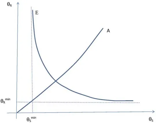
Equation ()defines an implicit function for in terms of that begins at the
origin and then is increasing everywhere as depicted in Figure 1. Intuitively, when the for-sale market is tighter, vacant houses are sold faster on average. Putting up a house for sale then should yield greater expected discounted returns. For the no-arbitrage condition to continue to hold, the expected discounted returns of putting up a house for rent have to increase in tandem, which comes about when the rental
market is tighter too. Equation()defines another implicit function for in terms
of which is everywhere decreasing, as depicted in Figure 1. The interpretation is
that in a tighter for-sale market, there will be faster sale on average, leaving behind fewer vacant houses for sale. In this case, there have to be more vacant houses for
rent for the supply of vacant houses to be just equal to −1. There can be more
rental vacant houses on the market only if the houses are rented out more slowly on average due to a smaller instantaneous probability of lease as in a slower market with a smaller.
It should be clear from Figure 1 that the two functions()and()must intersect
once and only once, meaning that there is aunique pair of{,}that solves the two
equations.25 Once the two market tightness are pinned down, the various equilibrium
expected returns, the sale price, the market rental, and the measures of households and vacancies in the two markets are known given that they can all be shown to be functions of {, }.
Before proceeding further, we would like to argue that the two equilibrium
condi-tions ()and() are both rather compelling. If condition()fails to hold, then no
vacant houses would be made available for sale or for rent, depending on whether
Figure 1: Existence and uniqueness of equilibrium
falls below or exceeds. In particular, suppose initially; then the tightness
of the for-sale market should reach infinity as all owners of vacant houses shun the
market. But then if the market were that tight, the sale price and then the
ex-pected discounted returns of putting up a house for sale should rise significantly to
overtake the initially greater expected returns . This kind of oscillation, if it ever
takes place at all, should eventually settle down when = just holds. Condition
() which stipulates that the sum of the vacancies in the two market + is
equal to the stock of vacant houses −1 is a straightforward adding-up constraint,
the violation of which gives rise to a logical inconsistency of thefirst order.
2.3
Empirical Implications
Our main goal in studying a model of a frictional housing market is to analyze how the transaction volume in the for-sale market and the rent-to-price ratio are determined simultaneously and how the two may be correlated in the time series and in the
cross section. At this point, it helps to simplify to assume that () = ();
i.e., there is the same matching function for the for-sale and the rental markets. This is a reasonable assumption, as there should not be any reason to believe the
matching technologies in the for-sale market and the rental market should differ in
2.3.1 Transaction Volume
In the for-sale market, there is a stock of vacant houses on the market at each
moment in time, each one of which is sold at the instantaneous probability ().
Then, over a unit of time, there would be
=() (19)
houses sold in the market.
Proposition 2 The transaction volume in the for-sale market is increasing in, and .
Proof. Solving(14)-(18) for and then substituting into (19),
=
() () +
(20)
which is increasing in and but decreasing in.
First note that () holds only if for () =(). Then, an increase
in lowers the LHS of(), which must be followed by decreases in and/or for
the condition to be restored. An increase in must similarly be met by decreases
in and/or for () to continue to hold. By(), the two market tightness goes
up and down together. Then an increase in or must be met by a decline in .
Thus, is increasing in by the direct effect of a larger and the indirect effect of
a smaller, whereas is increasing in by the indirect effect of a smaller .
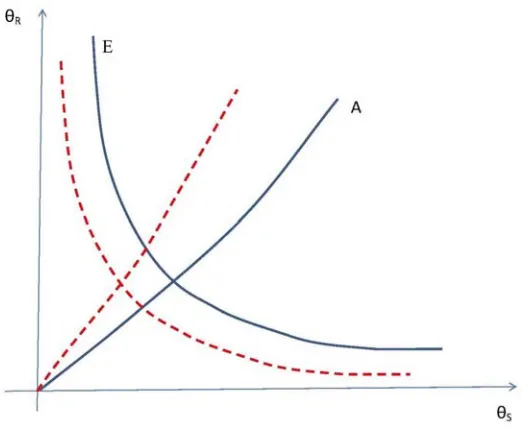
An increase in lowers the LHS of (), meaning that there has be to a smaller
for each for the condition to hold, as depicted in Figure2. It is straightforward
to verify that with a larger , there is a larger for each for () as depicted in
Figure 2, given that in equilibrium. Now, either tendency gives rise to a
smaller as can be seen in Figure 2. , as given in (20) then increases by the
direct effect of a larger and the indirect effect of a smaller
That there should be a greater volume of sales in a market with a larger housing stock and where a larger fraction of households demand for-sale housing is perhaps not
surprising. Holding and constant, the Proposition says that there would also be
a greater sale volume when there is a higher matching probability with which more
meetings between pairs of buyers and sellers result in successful sales. But notice that when houses are sold more quickly, there can only be fewer vacant houses left behind,
other things equal. Yet, with the housing stock given, there must be the same
stock of vacant houses on the market. The apparent contradiction is resolved once it
is recognized that when mismatched households spend less timefinding suitable new
Figure 2: Comparative steady states of
houses on the market. In all, with a greater matching probability , more houses are
put on the market for sale and more such houses are sold at each moment in time. An empirically more relevant question is how the normed transaction volume
may vary with the environment rather than how itself varies. Of course, if
is increasing in and , is increasing in the two exogenous variables too.
However, need not be increasing in even if is increasing in. Intuitively,
with the same population of households demanding for-sale housing but a greater housing supply, there should be fewer houses sold per unit of the housing stock.
Conjecture 3 The normed transaction volume in the for-sale market is
de-creasing in .
In a wide variety of quantitative analyses that we undertake, we find the
Conjec-ture indeed always holds.26
2.3.2 Sale Price and Market Rental
We next turn to the determination of the sale price and market rental. Solving
(3)-(13), we find that
= +() (2+ 2+())
(21)
26The analyzes assume
() =() = for some 0and ∈(01). The computer codes
= (++()) (+()) +() (++())
2 (22)
Proposition 4 The sale price is decreasing in and . The market rental is
decreasing in and if .
Proof. The sale price , as given in (21), is increasing in . The market rental
as given in(22), is guaranteed increasing in if . The two market tightness
is decreasing in and, as shown in the proof of Proposition 2.
With a larger housing stock, there would more for-sale vacant houses on the market
and a more sluggish market follows. Sale pricethen falls as the market slows down.
The reason for howshould be decreasing intoo is as follows. First observe that
in equilibrium from(), which results from the difference in the bargaining
environment facing agents in the two markets. In the for-sale market, the surplus
of a match is equal to −f, independent of the sale price and the value of a
vacant unit . That the sale price — a transfer between the buyer and the seller — is
not part of the surplus is not surprising. More subtle is that the value of a vacant
unit is also not a factor, which is the result of the effect of the seller forgoing a
vacant unit and the effect of the buyer becoming an owner of one cancelling out. In
the rental market, the surplus of a match is − in addition to −e, the latter
roughly equal in value to −f in that the gains to both the rental household
and the owner-occupier by becoming matched are equal to the PV of the flow payoff
. Apparently, there tends to be a larger surplus in the rental market than in the
for-sale market, other things equal. In the rental market, when a match takes place,
the owner of the previous units occupied by the rental household suffers a capital loss
−e. This loss can be thought of as an externality as it is not taken into account
in the bargaining between the rental household and his new landlord. Had it been
considered by the agents, the loss would have canceled out the gain −. All this
then tends to cause to exceed for the same market tightness. The no-arbitrage
condition thus requires a tighter for-sale market to equalize and. In this case,
given and, transferring one household from the less tight rental market to the
tighter for-sale market raises the overall market tightness and therefore lowers the
overall measure of vacant houses + from the previous level. To restore the
equality in () requires a decline in market tightness in one or both markets. But
since, by the no-arbitrage condition(), the tightness in the two markets must move
in the same direction, and decline in tandem, where the decline in the former
causes to go down.
In the meantime, in a slower market, there will not just be more houses for sale, but also more houses for rent as well. Then, perhaps the market rental should also
go down too in response to either a decline in or. Surprisingly, it does not seem
possible to ascertain such a tendency without further assumptions. The present setup
after the match between the household and house is broken while the household is searching for a new house. In a slower market, on average, a new match is found
sooner. This raises the renter’s surplus from entering into the lease in thefirst place,
knowing that on average he/she is only obliged to continue paying the same rent for a shorter period of time after the newly found house no longer matches his/her need.
It cannot be ruled out in general that this effect dominates the direct negative effect
of a slower market on equilibrium rental unless . In some extensive quantitative
analyses, however, we have not uncovered a single instance where indeed becomes
increasing in or even for ridiculously large . In all, it seems safe to conclude
that an increase in the two variables should also lower, in addition to loweringfor
any practical values of.
We next move to check how and should vary with . First, notice that
by (21), holding constant and therefore the instantaneous meeting probabilities
() and (), the sale price is increasing in — other things equal, a higher
matching probability means that mismatched houses, when they can be sold faster on average, are more liquid assets commanding a higher sale price. In the meantime
though, a higher matching probability would be followed by a decline in to meet
the restrictions in(), which tends to lengthen the time mismatched houses can be
sold, turning them into less liquid and therefore less valuable assets. Our quantitative
analyses indicate that the direct positive effect dominates for smallbut the indirect
negative effect dominates for large ; i.e., is initially increasing but eventually
decreasing in. Intuitively, whenis large to begin with, there tends to be a relatively
small initial. With a concave function, for the relatively small initial, a given
decline in results in a large decline in(). In this way, the instantaneous sale
probability () tends to be decreasing in for large.
Not unexpectedly, a similar initially positive and eventually negative effect of is
also found on market rental in our quantitative analyses.
Conjecture 5 The sale price and the market rental are both initially increasing
but eventually decreasing in .
2.3.3 Rent-to-Price Ratio
Dividing(22) by (21) and making use of(),
=
µ
+() +()
() ()
+ ()
(++()) (+())

(23)
Other things equal, owners should require a rental yield above the discount rate to
willingly offer his/her property for rent instead of for sale given that a rental unit
would earn no rental income every now and then when the unit becomes vacant. The
above equation indeed says that is guaranteed to hold if() =()as
By Proposition 4, increases in or cause to decline for sure and should also
lead to a smaller. How the rent-to-price ratio should behave then depends on how
the elasticities ofcompare against the elasticities ofwith respect to and. Our
conjecture is that thefirst set of elasticities should be greater than the second set. A
larger or causes and to vary through the changes in the respective market
tightness in the two markets. In the rental market, as we argue above, an increase
in has both a usual positive and an indirect negative effects on , whereas in the
for-sale market, there is just the usual positive direct effect of on . If indeed
decreases proportionately more thandoes in response to a given increase in or,
to follow is a larger. The conjecture holds up always in our quantitative analyses.
The ratio , given in (23), is guaranteed to be decreasing in for small
and/or, holding constant the two market tightness, meaning that an increase in the
matching probability, other things equal, tends to exert stronger positive effects on
the sale price than on the market rental. This is reasonable in that an improvement in asset liquidity should mainly help raise the sale price, whereas the market rental
should not directly benefit from the improvement.
The rent-to-price ratio can also vary in response to the given increase in to
the extent that the increase in impacts on the two market tightness, on which
and depend. By Conjecture 5, an increase in should cause both and to go
up initially but to fall eventually as the two market tightness decline. Along the
increasing phase, should increase proportionately more than does, just as rises
faster than in response to a given decline in or In this case then, should
fall. Along the decreasing phase,should decrease proportionately more thandoes,
to which a larger should follow. In our quantitative analyzes, however, we find
that is everywhere decreasing in . Apparently, any tendency for to increase
with arising from the changes in market tightness is more than offset by the direct
negative effect of on.
Conjecture 6 The rent-to-price ratio is increasing in and but decreasing
in.
In sum, varies in the way it does as described in the Conjecture is due to the
tendency that the sale price should be more sensitive to changes in market tightness
arising from changes in supply and demand composition and that improvements
in market liquidity should help raise the sale price more than the market rental.
2.3.4 Correlation between the Transaction Volume and Rent-to-Price ra-tio
Proposition 2 and Conjecture 6 together imply that:
Corollary 7 Variations in induce a positive correlation between and ,
i.e.,
Variations in induce a negative correlation between and , i.e.,
( )0 (25)
Conjectures 3 and 6 together imply that:
Corollary 8 Variations in induce a negative correlation between and ,
( )0 (26)
By construction, the housing units in the model are observationally identical and as such the model has no cross-sectional implications. But then, if we imagine,
instead of there being one unified housing market, that there are numerous segmented
markets, each of which is as described in the model above. The theoretical results can then be interpreted as cross-sectional implications. The last two Corollaries suggest that across the segmented markets, transaction volumes and the rental yields can exhibit negative correlations or positive correlations. Our empirical analyses in the following are in the main motivated to resolve this ambiguity of the theoretical
model.27
3
Our Econometric Framework
In this section, we describe our econometric framework for testing the predictions of the theoretical model with a cross-sectional data set. In particular, we test whether a
change in the fraction of owner-occupants, or in the probability of good matchor
in the housing stock would induce the rent-to-price ratio()and the transaction
ratio in the sale market () to move in the same or opposite directions. Two
issues need addressing to achieve these goals. First, in the model, housing units are homogeneous, while in practice they are heterogeneous. Second, we must also obtain
a measure of the probability of good match which would vary across different
sub-markets (which are REDs in the current context). One possible method is to adopt a hedonic-type regression in order to control for the heterogeneity among housing
units. Unfortunately, is not directly observable. In addition, as our sample size is
relatively small (132 RED), listing all the control variables on the right hand side
of the regression equation would exhaust our degree of freedom, and adversely affect
subsequent analysis. Therefore, a hedonic-type regression approach is not practical.
Another common approach is to use principal component (PC) analysis, which
“com-bines” different variables into a few “factors” or PCs. We can then use those PCs
as the right hand side variables to control for differences across RED. However, a
prerequisite of adopting the PC analysis is that those variables are significantly
cor-related, and that a few variables can summarize most of the total variations (Jolliffe,
2005). Unfortunately, this is not the case in our sample. It takes six PCs to account for 80% of the total variations, as shown in the appendix, and hence adopting the PC analysis would not be helpful in our context. Furthermore, neither the hedonic nor
PC approach provides an empirical proxy for An alternative approach is required.
The starting point of our approach is the observation thatvariations in the fraction
of owner-occupants, in the probability of good match and in housing attributes can be
interpreted as changes in particular popularity measures. For instance, a RED that
is more popular (i.e. has some good features) would attract more owner-occupants. Since owners tend to stay longer than renters, we would observe less turnover on average. On the other hand, a RED with a high matching probability means that, other things being equal, the housing units are more liquid. This attracts investors and increases the popularity of the RED. Similarly, as the number of households
targeting each submarket is normalized to unity, can be interpreted as the relative
demand for housing in a certain submarket. Thus, the smaller is, the stronger
the relative demand for residence in a particular submarket. Obviously, the more desirable the structural and neighborhood attributes are, the greater the demand
for the RED, and hence a smaller and a higher popularity. Accordingly, we can
summarize the major implications of the search and matching model (from (24) to (26)) as follows:
()
( ) ≷0,
()
( ) ≷0. (27)
As the theoretical analysis does not help us to dictate the relationship, we switch
to the empirical analysis. Thus, our next step is to build acomposite popularity index
based on housing affordability and a bundle of structural, neighborhood, and location
characteristics. A significant advantage of this approach is that we consolidate the
information that are contained in the structural and neighborhood characteristics of a RED into one variable, hence we can increase the degree of freedom in our regression. Thus, the “popularity” index can be interpreted as a “summary statistics” of many housing characteristics as well as a “proxy” for the matching probabilities which we do not observe directly, and therefore it needs to be inclusive. Our choice of the
“ingredients” of the popularity index is influenced by the hedonic pricing literature,
motivated by exploratory interviews with market practitioners,28 and constrained by
data availability. Following a large literature on index construction, our popularity
index is a linear sum of equally weighted selected indicators.29 We provide more
details about the construction of the index in a later section and in the Appendix. It is clearly an imperfect proxy of the conceptual “popularity” in the model. Even if we were able to include all of the characteristics of a RED in the index, it is unlikely it could address all the concerns surrounding relative demand and the likelihood of a successful match, which result from the interactions of consumers with the housing market (Griliches 1971).
If we take the existence of a popularity proxy for granted, a natural formulation
reflecting the simultaneous relationship between the rent-to-price ratio () and
the transaction rate () on one side, and how both variables may relate to the
Popularity index on the other is:
= 0 +1( ) +2 µ

++1
= 0+1( ) +2 µ

++2 (28)
where and are row vectors of other controls, whose detailed contents will be
discussed later. , , = 012 are all scalars, while and are column vectors.
1 and 2 are residual terms. In line with the model implications, we should expect
1 0, 1 0, 2, 2 0 In words, it means that we expect more frequent
trading in popular REDs. And the rental yield must be lower to compensate for higher popularity. Clearly, this simple simultaneous equations system (28) can be rearranged as µ 
= 0
0+01( ) + (+2) + (1+22)
µ

= 0
0+01( ) + (2+) + (21+2) (29)
where = (1−22),00 =0+20,01 =1+21,00 =0+02,01 =1+12
Several issues emerge. Clearly, () is correlated with1, and() is correlated
with 2. Thus, there are “cross-equation restrictions” implicitly imposed in (28),30
and if we estimate each equation in (28) separately, the ordinary least squares (OLS)
estimates are inconsistent. Similarly, even though 1 and 2 in (28) can be assumed
to be independent error terms, (1+22) and (21+2) in (29) are clearly not
29Notice that while some of our indicators are continuous variables, some are dummy variables. And without any prior knowledge of the detailed preference of the households, we consider the choice of using an equal-weighted linear sum of different indicators to be both sensible and consistent with the practice of the literature on index construction.
independent. Again, it is a kind of “cross-equation restriction.” Thus, ignoring such a restriction and estimating the two equations in (29) separately with OLS may not
deliver efficient estimates, as the covariance between(1+22) and (21+2) are
not properly taken into considerations. In this case, structural estimators should be
preferred. More specifically, we use 3SLS, which is a full information estimator, and
estimate the two equations as a system.31 The procedure is as follows:
Stage 1
µ

= 0+1( ) +++1
µ

= 0+1( ) +++2
where 0, 1, 0, 1 are scalars, and , , , are vectors. We obtain the OLS
projections of the endogenous variables, ³d´ and¡[
¢ Stage 2 µ 
= 0+1( ) +2
\
µ

++1 (30)
µ

= 0+1( ) +2
d µ

++2 (31)
where , are vectors. We retain the residuals to form a consistent estimate of the
covariance matrix of the disturbances. Stage 3
Perform Generalized Least Squares (GLS) estimation on (30), (31) with the covariance matrix in Stage 2 as the optimal weighting matrix. For the future reference, (30) would be labelled as the rent-to-price equation, and
(31) as the turnover equation.
4
Data and Popularity Index construction
In this paper, we use data from three different sources. First, we retrieve
micro-transaction records from EPRC, a commercial Hong Kong real estate database. Sec-ond, we obtain demographic and socioeconomic data from the 2011 Hong Kong Cen-sus. We also use online resources, including real estate brokers’ and government web-sites, geographic information system, and popular local internet discussion forums,
which provide us with complementary information on structural, neighborhood, and locational characteristics.
The EPRC data set has been employed by several previous studies.32 We therefore
first discuss the official census. To gain a better understanding of the socioeconomic
environment, the Hong Kong government conducts a census of all households in Hong Kong every decade, and a by-census for a selected sub-sample between the main cen-suses. Previous censuses and by-censuses published at most the district level data for
public reference.33 In the 2011 Census, the Census and Statistics Department (CSD)
of the Hong Kong government provides publicly accessible statistics of “major hous-ing estates,” (i.e. REDs) “with at least 3,000 residents or 1,000 domestic households”
at the time of survey.34 Information is readily available for a total of 487 REDs (or
“estates”), of which 163 are private residential REDs. We exclude all public housing, as the allocation of these units is not decided by the market and the corresponding rents and prices are highly subsidized. This collection of private residential RED is far from being ideal, but it does provide information on demographics, income and housing related expenditure disaggregated at the RED level. Hong Kong has no zip code system, but as most of the Hong Kong population lives in high-rise buildings, the RED level analysis in Hong Kong can be comparable to those zip code-level analyses of the US. We include variables for the total population, the young population aged from 25 to 44 years, the percentage of residents’ with a college education, the house-hold monthly median income, the median monthly mortgage payment, and residents working in real estate consulting industry.
The 2011 Census was conducted from June 30 to August 2, 2011. Correspondingly, we extract rental contracts, as well as “purchase and sale agreements” (i.e. contracts of for-sale housing units) from EPRC that occurred in the 163 private REDs in the
subsequent period. Typically, a transaction is completed in two months; hence we
restrict the time horizon to range from November 2011 to October 2012.35 For each
RED, we are able to observe the actual transaction volume. With some data cleaning
efforts, we collect 3,616 transactions in the rental market and 29,671 transactions in
the for-sale counterpart.36 Notice that in any given period of time, a housing unit is
either transacted in the sale marketor the rental market,but not both. Therefore, to
find the rent-to-price ratio while holding the quality of the housing unit constant, we
32Among others, see Leung et al. (2002).
33There are eighteen administrative districts in Hong Kong. For a list of these districts, please visit the District Council homepage http://www.districtcouncils.gov.hk/index.html .
34The official webpage is http://www.census2011.gov.hk/en/major-housing-estates.html.
35Notice that the data set is constructed in a manner that the potential simultaneous bias is mitigated. According to Leung, Leong and Chan (2002), most housing transactions in Hong Kong are finished within two months. Therefore, when we collected housing transactions between November 2011 to October 2012, even the initial sale agreements were signed after the 2011 Census wasfinished, and hence we can take the variables from the household survey as “pre-determined” variables. For more justifications on using pre-determined as exogenous variables, see Greene (2008), Sims (2010).
need to match each transaction from the rental market with one in the sale market
with “similar characteristics.”37 Following Huang and Leung (2014), we require the
unit for-sale and the unit for rental both to be transacted in the sampling periods,
and to have the same estate code,floor level, living room orientation, the gross square
footage to differ by not more than ten feet, the net gross ratio to differ by less than
one percent, and to have a building age