Heuristic Switching Model and Exploration Explotation Algorithm to describe long run expectations in LtFEs: a comparison

Munich Personal RePEc Archive

Heuristic Switching Model and

Exploration-Explotation Algorithm to

describe long-run expectations in LtFEs:

a comparison

Colasante, Annarita and Alfarano, Simone and

Camacho-Cuena, Eva

Universitat Jaume I

2019

Online at

https://mpra.ub.uni-muenchen.de/92391/

Heuristic Switching Model and

Exploration-Explotation Algorithm to describe

long-run expectations in LtFEs: a comparison

Annarita Colasante, Simone Alfarano, Eva Camacho-Cuena

Universitat Jaume I

Abstract

We compare the performance of two learning algorithms in replicating individual short and long-run expectations: the Exploration-Explotation Al-gorithm (EEA) and the Heuristic Switching Model (HSM). Individual expec-tations are elicited in a series of Learning-to-Forecast Experiments (LtFEs) with different feedback mechanisms between expectations and market price: positive and negative feedback markets. We implement the EEA proposed by Colasante et al. (2018c). Moreover, we modify the existing version of the HSM in order to incorporate the long-run predictions. Although the two algorithms provide a fairly good description of marker prices in the short-run, the EEA outperforms the HSM in replicating the main characteristics of individual expectation in the long-run, both in terms of coordination of individual expectations and convergence of expectations to the fundamental value.

JEL:D03,G12,C91.

1

Introduction

The origin of heterogeneity across individual expectations and the role that it plays in shaping aggregate outcomes is an important topic in theoretical as well as empirical research in macroeconomics. Expectations, however, are not directly observable, differently from prices of stocks, volumes of sold books, interest rates of bonds, downloads or number of likes, which can be precisely measured and recorded in the new world where almost “everything” is now in electronic format. This means that there is a significant limitation when it comes to fully understanding the precise role played by expectations in driving macroeconomic aggregates. One way to circumvent this problem and rigorously model the expectations of individuals is to assume consistent expectations, i.e. rational expectations, following the seminal idea of Muth (1961) which has been further developed by Lucas Jr and Prescott (1971). From a formal point of view, the main advantage of rational expectations is that agents can be rational in one way only. The argument put forward by Friedman (1966) on the irrelevance of “irrational” individuals in the long-run gives to the rationality assumption a further intuitive appeal.

As an alternative to the rational expectations paradigm, it certainly plays a central role the bounded rationality assumption of economic agents, introduced by Simon (1957). In the world of bounded rational agents, we typically loose the uniqueness of the behavior, since agents can be “non-rational” in many different ways. In order to shed some light on the degree of bounded rationality of indi-viduals, laboratory experiments have been largely demonstrated to be an essential methodology. Countless experiments have repetitively shown that in complex en-vironments, subjects follow simple adaptive rules, called heuristics, in order to form expectations, changing their mind as a function of the evolution of the en-vironment and adapting to the new circumstances. The principle of anchor and adjustment, introduced by Kahneman and Tversky (1973), is a sufficiently general and flexible framework that can be certainly cast into the bounded rationality paradigm and able to realistically describe the way individuals form and adapt their expectations.

short-run expectations in different economic environments: in financial markets (Hommes et al. (2005)), real estate markets (Bao and Ding (2016)), commodity markets (Bao et al. (2013)) and in simple macroeconomic frameworks (Assenza et al. (2011); Anufriev et al. (2013); Cornand and M’baye (2016)). The vast

ma-jority of those LtFEs focuses on eliciting individual short-run expectations, i.e.

providing incentives to forecast the next period market price. The novel contri-bution to this experimental literature of Colasante et al. (2018a,b) is to focus on the entire spectrum of expectations, since they elicit contemporaneously short and

long-run expectations about the evolution of the market price under positive and

negative feedback systems. In particular, they explicitly give incentives to the subjects to submit their predictions on the market price at the beginning of every period, giving the possibility to revise the predictions as new information becomes available. This experimental design allows to study how expectations form and co-evolve with the price at different forecast horizons. Their results concerning short-run predictions are in line with the literature (see Heemeijer et al. (2009)): fast convergence and slow coordination in the markets with negative feedback, whereas slow convergence and fast coordination in the markets with positive feed-back. Regarding the long-run predictions, Colasante et al. (2018a,b) observe that in markets with positive feedback treatments the market price plays a pivotal role in the expectations formation process, whereas in markets with negative feedback it turns out that subjects use the fundamental value as their main reference point. We can find in the literature only few computational learning algorithms to describe individual expectations in LtFEs (see Heemeijer et al. (2009); Assenza et al. (2011); Bao et al. (2013); Hommes and Lux (2013)). The most commonly used is the so-called Heuristic Switching Model, HSM hereafter (see Brock and Hommes (1998)). Using experimental data on long-run expectations, Colasante et al. (2018c) have introduced an alternative adaptive learning model of bounded rationality, the Exploration-Exploitation Algorithm (hereafter EEA) that, con-trary to the HSM, accounts contemporaneously for subjects’ short- and long-run expectations.

characteristics of the analysed algorithms in an more efficient architecture, to de-scribe the date and model expectations.

The paper is organized as follows: in the Section 2, we illustrate the experimen-tal setting of the LtFE and the experimenexperimen-tal results. In Section 3, we describe the details of the two learning algorithms, namely the HSM and its modified version and the EEA. In Sections 4 and 5, we describe the simulation results and propose a modified version of the EEA to include a different anchor, respectively. Finally, in Section 6 we present the main conclusions.

2

The Learning to Forecast Experiment

2.1

Experimental Design

This paper builds upon the Learning to Forecast Experiments of Colasante et al. (2018a,b). In this section we briefly describe their novel experimental design to elicit subjects’ expectations at different time horizons. In those LtFEs the authors elicit subjects’ short and long-run expectations in markets characterized by either a positive or a negative expectations feedback system. They conduct a total of 15 sessions: 7 with positive and 8 with negative feedback. In each session, 6 subjects play the role of professional forecasters for 20 periods. More precisely,

at the beginning of period t, subject i submits her short-run prediction for the

price at the end of period t, denoted as ipet,t, as well as her long-run predictions

for the price at the end of each one of the 20−t remaining periods, denoted as

ipet,t+k, with 1 ≤k ≤ 20−t. To compute the market price, it is implemented the

pricing equation proposed by Heemeijer et al. (2009). In the positive feedback treatment, the law of motion of the price is given by:

pt=pf + 1

1 +r(¯p

e

t,t−pf) +ǫt, (1)

while in the negative feedback treatment the realized market price is computed as follows:

pt =pf − 1

1 +r(¯p

e

t,t−pf) +ǫt, (2)

where r= 0.05 in all sessions and pf is the constant fundamental value in a given

session.1

The term ¯pe

t,t in the equations is the average of the six one-step-ahead

1

To avoid the effects of communication among subjects between sessions, two different values forpf are implemented, so that there are some markets with a fundamental value equal to 65 and

others with a fundamental value equal to 70. In the positive feedback treatment, the fundamental value is computed aspf = d_r, where the average dividenddis equal to 3.5 or 3.25, depending on

predictions submitted at the beginning of period t, ¯pe

t,t =

1 6

P6

i=1ip

e

t,t. Finally, the

term ǫt∼N(0,0.25) is an iid normal shock.

The main difference between eqs. (1) and (2) is how expectations affect the price: eq. (1) describes a positive feedback system where subjects predictions are self-fulfilling, i.e. the higher (lower) is the average forecast, the higher (lower) will be the price. Eq. (2) describes, instead, a system in which there is a negative feed-back between expectations and price, i.e. the higher (lower) is the average forecast, the lower (higher) will be the price. Even if market price is solely determined by short-run predictions, all predictions are rewarded. Individual earnings at the end

of each period depend on forecasting errors and are computed as iπt =iπts+iπlt,

where iπst denotes the pay-off for the short-run predictions:

iπts =

250

1 +βi,t

with βi,t =

ipet,t−pt

2

2

. (3)

andiπtldenotes the subject’s pay-off that depends on her long-run predictions error,

being iπtl =

Pt−1

j=1 iπtl−j,t, where iπ

l

t−j,t represents the individual profit associated

with the prediction submitted by subject iat the beginning of periodt−j for the

price in period t, where 1 ≤ j ≤ t−1. The long-run predictions are rewarded

according to the following scheme:

iπtl−j,t =



    

    

25 if 0≤iδt−j,t ≤5

12 if 5<iδt−j,t ≤10

5 if 10<iδt−j,t ≤15

0 otherwise

(4)

where iδt−j,t =|ip

e

t−j,t−pt|. Note that subjects receive an immediate feedback on

their short-run forecasting accuracy, while they experience a delay in evaluating the accuracy of their long-run predictions. The final payment of each subject is the

sum of pay-offs across all periods.2

In the positive feedback treatment, subjects

are informed about the value of the constant interest rate (r), average dividend

(d), the asset prices until period t−1 and all their own (short and long-run) past

predictions. In the negative feedback, subjects receive only information about their own past predictions and the past market prices. As it is typically done in the literature of LtFEs, the subjects receive some qualitative information on the feedback system affecting the price mechanism and the profit functions. See Colasante et al. (2018a,b) for additional details about the experimental design.

2

The parameters of the pay-off functions are calibrated such that approximately maxP20

t=1iπts = max

P20

t=1iπlt, in order to give to the subjects the same incentive to provide

According to eqs. (1) and (2), the REE predicts that the price pt converges to the fundamental value with fairly small fluctuations proportional to the

idiosyn-cratic shock term ǫt. What would be the REE for long-run expectations? When

eliciting their long-run expectations, subjects submit at the beginning of period t

their predictions for the end of period t+k, for all k >0. The price at the end

of period t+k is a function of the subjects’ short-run predictions submitted at

the beginning of period t+k. Each subject has, indeed, to guestimate k-periods

in advance, the short-run predictions of the other subjects. If we assume that all

subjects follow rational expectations, then their predictions in each period t and

for each forecast horizon k are are ipet,t+k ≈pf, independently of the expectations

feedback system.

2.2

Experimental results

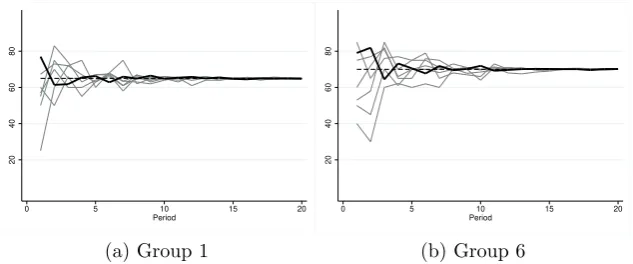
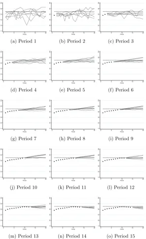
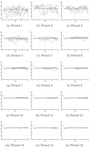
In the following we summarize the experimental results in Colasante et al. (2018a). Figure 1 displays the dynamics of the market price in all the 15 markets. As an illustrative example, Figures 2 and 3 show the individual short-run predictions and the market price dynamics in two representative group for each treatment. From a visual inspection of those figures, we observe that market prices follow qual-itatively different patterns, depending on the feedback mechanism implemented in the particular treatment. In the positive feedback treatment, short-run pre-dictions coordinate after few periods, although not necessary to the fundamental value. The market price exhibits an oscillatory pattern without converging to the fundamental value. In the negative feedback treatment, instead, we observe that market prices quickly converge to the fundamental value after few periods of uneven fluctuations, while individual short-run predictions need more periods to coordinate on the fundamental value. Figures 4 and 5 show individual long-run predictions in two representative groups, one for the positive and one for the negative feedback treatment, respectively.

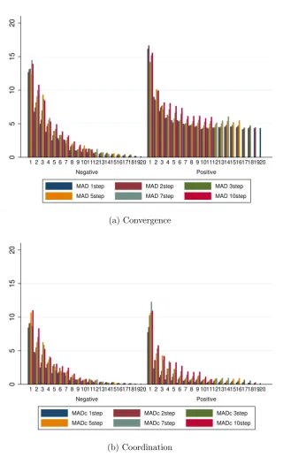
To quantify the convergence of the expectations, the Mean Absolute Deviation (MAD) between individual predictions and the fundamental value is computed for both, short and long-run predictions as:

M ADpf

t,t+k =

* P6

i=1|ipet,t+k−pf|

6

+

g

, (5)

with k=0,1,2,4,6,9. The notation < ... >g denotes the average across groups. To

quantify the degree of coordination, the MAD between individual predictions and

the (within-group) average predictions is computed for each period t and for a

40

50

60

70

0 5 10 15 20 0 5 10 15 20

pf = 65 pf = 70

Period

(a) Positive feedback

60

65

70

75

80

0 5 10 15 20 0 5 10 15 20

pf = 65 pf = 70

Period

(b) Negative Feedback

Figure 1: Realized price for all groups in the two treatments. The blue solid lines are market prices, the dashed lines represent the fundamental value.

40

60

80

0 5 10 15 20 Period

(a) Group 1

40

60

80

0 5 10 15 20 Period

(b) Group 6

Figure 2: Realized price and individual short-run predictions of two representative groups in the positive feedback system. The black solid line is the market price, the grey lines are the individual one-step-ahead predictions and the dashed line represents the fundamental value.

M ADC

t,t+k =

* P6

i=1|ip

e

t,t+k−p¯et,t+k|

6

+

g

, (6)

20

40

60

80

0 5 10 15 20 Period

(a) Group 1

20

40

60

80

0 5 10 15 20 Period

(b) Group 6

Figure 3: Realized price and individual short-run predictions of two representative groups in the negative feedback system. The black solid line is the market price, the grey lines are the individual one-step-ahead predictions and the dashed line represents the fundamental value.

only in the negative feedback treatment, while, in the positive feedback treat-ment, predictions systematically deviate from the fundamental value. Focusing on coordination of expectations, in the positive feedback treatment, subjects’ one step-ahead predictions coordinate faster than in the negative feedback treatment, whereas in the long-run predictions, the forecasts disagreement increases with the horizon, i.e. the longer is the forecast horizon, the higher is the dispersion of predictions. This is strongly connected to the absence of a long-term anchor for subjects’ expectations. In fact, the long-run predictions are characterized by some sort of cone-shape trajectory, compatible with a linear trend extrapolation rule of subjects with heterogeneous slopes. In the negative feedback treatment, where sub-jects learn the fundamental value, coordination of short and long-run predictions occur simultaneously, driven by the converge of the market price to the funda-mental value. Subjects are able to learn the REE and, as a consequence, both price and expectations converge to it over time. It is just in the negative feedback system that the REE constitutes a good benchmark to describe the market price dynamics and the evolution of subjects’ expectations.

3

Learning Algorithms: HSM and EEA

In this section we describe the details of the two learning algorithms that we employ to reproduce the experimental data.

0 20 40 60 80 100

0 5 10 15 20 Period

(a) Period 1

0 20 40 60 80 100

0 5 10 15 20 Period

(b) Period 2

0 20 40 60 80 100

0 5 10 15 20 Period

(c) Period 3

0 20 40 60 80 100

0 5 10 15 20 Period

(d) Period 4

0 20 40 60 80 100

0 5 10 15 20 Period

(e) Period 5

0 20 40 60 80 100

0 5 10 15 20 Period

(f) Period 6

0 20 40 60 80 100

0 5 10 15 20 Period

(g) Period 7

0 20 40 60 80 100

0 5 10 15 20 Period

(h) Period 8

0 20 40 60 80 100

0 5 10 15 20 Period

(i) Period 9

0 20 40 60 80 100

0 5 10 15 20 Period

(j) Period 10

0 20 40 60 80 100

0 5 10 15 20 Period

(k) Period 11

0 20 40 60 80 100

0 5 10 15 20 Period

(l) Period 12

0 20 40 60 80 100

0 5 10 15 20 Period

(m) Period 13

0 20 40 60 80 100

0 5 10 15 20 Period

(n) Period 14

0 20 40 60 80 100

0 5 10 15 20 Period

(o) Period 15

20

40

60

80

100

0 5 10 15 20 Period

(a) Period 1

20

40

60

80

100

0 5 10 15 20 Period

(b) Period 2

0 20 40 60 80 100

0 5 10 15 20 Period

(c) Period 3

0 20 40 60 80 100

0 5 10 15 20 Period

(d) Period 4

0 20 40 60 80 100

0 5 10 15 20 Period

(e) Period 5

0 20 40 60 80 100

0 5 10 15 20 Period

(f) Period 6

0 20 40 60 80 100

0 5 10 15 20 Period

(g) Period 7

0 20 40 60 80 100

0 5 10 15 20 Period

(h) Period 8

0 20 40 60 80 100

0 5 10 15 20 Period

(i) Period 9

0 20 40 60 80 100

0 5 10 15 20 Period

(j) Period 10

0 20 40 60 80 100

0 5 10 15 20 Period

(k) Period 11

0 20 40 60 80 100

0 5 10 15 20 Period

(l) Period 12

0 20 40 60 80 100

0 5 10 15 20 Period

(m) Period 13

0 20 40 60 80 100

0 5 10 15 20 Period

(n) Period 14

0 20 40 60 80 100

0 5 10 15 20 Period

(o) Period 15

0

5

10

15

20

Negative Positive

1 2 3 4 5 6 7 8 9 1011121314151617181920 1 2 3 4 5 6 7 8 9 1011121314151617181920

MAD 1step MAD 2step MAD 3step MAD 5step MAD 7step MAD 10step

(a) Convergence

0

5

10

15

20

Negative Positive

1 2 3 4 5 6 7 8 9 1011121314151617181920 1 2 3 4 5 6 7 8 9 1011121314151617181920

MADc 1step MADc 2step MADc 3step MADc 5step MADc 7step MADc 10step

(b) Coordination

Figure 6: Convergence and coordination of short and long-run expectations in the positive and negative feedback treatments.

which constitutes a fitness measure to rank those rules. In every period, each subject selects the rules with a probability proportional to the fitness measure, so that the best performing rule has higher chances to be selected. Similarly to the HSM, the EEA is based on the very basic principle of anchor-and-adjustment, (Kahneman and Tversky (1973)). Differently from the HSM which can be thought as a “parametric” learning algorithm, the EEA allows a higher degree of flexibil-ity in the range of possible prediction rules, see Colasante et al. (2018c). Its key learning mechanism is the identification of the range of feasible actions around the anchor, represented by the market price in the previous period. As long as more information on the price dynamics is available, each subject adjusts her own range of possible predictions and, then, selects her specific prediction proportion-ally to the fitness measure. The process of selection consists of two main phases: the exploration phase, in which subjects have few information and try to form their expectations about the future evolution of the market price; the exploitation phase, in which subjects refine their predictions in order to locally “optimize” their performance. Note that in the EEA we are not imposing any precise parametriza-tion of the subjects’ predicparametriza-tions, which are free to vary in a range whose evoluparametriza-tion adapts to the past market conditions.

3.0.1 The Heuristic Switching Model

In the following, we list the four heuristics of the HSM as introduced by Bao et al.

(2012). We label the four rules according to the index h = 1, ..,4, indicating the

corresponding forecasting price as hpet,t. Note that the left sub-index h denotes

now the heuristic instead of the subject. The heuristics are3

:

• Adaptive rule (ADA):

1pe_t,t=αpt−1+ (1−α)p

e

t−1,t−1 0< α <1. (7)

• Trend following rule (TFR):

2pe_t,t =pt−1+w(pt−1 −pt−2) w >0. (8)

• Contrarian rule (CR):

3pe_t,t=pt−1+s(pt−1 −pt−2) s <0. (9)

• Learning and adjustment rule (LAA):

4pe_t,t= 0.5(pav_t−1+pt−1) + (pt−1−pt−2)

3

The learning mechanism is based on the possibility for the subjects to switch among the four given rules, choosing the one providing the relatively highest prof-itability in the recent past. The following equation is employed to compute the performance of each heuristic:

Uh,t−1 =−

pt−1−hpet−1,t−1

2

+η Uh,t−2, h= 1, ...,4,

where the parameter 0 ≤η ≤ 1 represents the “memory” of agents, meaning the

weight assigned to past errors. We set η= 0.7, following Hommes (2013).

It is assumed that only a fraction of agents changes their rule every period. The share of agents using a specific rule is computed by using the discrete choice model with asynchronous updating as in Diks and Van Der Weide (2005):

nh,t =δ nh,t−1+ (1−δ)

exp(β Uh,t−1)

Zt−1

, (10)

Zt−1 = 4

X

h=1

exp(β Uh,t−1), (11)

where 0< δ ≤1 denotes the share of agents that update their choice; the

param-eterβ ≥0 represents the intensity of choice and it determines the switching speed

to the most successful rule. Zt−1 is a normalization factor. As in Hommes (2013),

we consider δ = 0.9 and β = 0.4. We compute the expected price as a weighted

average across the different expectations given by the four rules:

¯

pe

t,t =

4

X

h=1

nh,t−1 hp e

t,t.

Plugging the value of ¯pe

t,t into eqs. (1) and (2), we compute the market price, in

the positive and negative feedback treatment, respectively.

We generalize the HSM in order to account for the long-run expectations. We simply assume that the subjects linearly extrapolate their short-run prediction rules to determine their long-run expectations as follows:

• Long-run adaptive rule (L-ADA):

1pe_t,t+k =pt−1 + (k+ 1) α(pt−pet−1,t−1) k = 1,2,3. (12)

• Long-run trend following rule (L-TFR):

• Long-run contrarian rule (L-CR):

3pe_t,t =pt−1+ (k+ 1) s(pt−1−pt−2) k = 1,2,3.

• Long-run learning and adjustment rule (L-LAA):

4pe_t,t= 0.5(p_tav₋1 +pt−1) + (k+ 1)(pt−1−pt−2) k= 1,2,3.

We assume that, once an agent selects one of the short-run prediction rules, she extrapolates linearly that rule in order to predict prices in horizons up to 4-steps

ahead. In other words, we assume that the selection of the rule at timet is based

on the feedback from the profits associated to the short-run predictions only. Our simple modification of the HSM to account for long-run predictions is the first step in this direction present in the literature on LtFEs. It is essentially based a simple intuition and in its easy implementation.

3.0.2 The EEA: the Exploration-Exploitation Algorithm

The Exploration-Exploitation Algorithm, as outlined in Colasante et al. (2018c), is a non parametric learning algorithm implemented to characterize the price dy-namics of both, short- and long-run expectation in LtFEs. We assume that each subject, represented by and artificial agent, has a set of available actions in ev-ery period. To compute short-run predictions, the range of action of the artificial agents evolves adaptively as a function of the past price and expectations. In particular, the range of the set of actions is centred in the last realized price and its range, which represents the exploration space, is proportional to the standard deviation of the past market prices. The probability to take a particular action is proportional to a given distribution, with mean computed as a convex combina-tion between the last observed price and its past prediccombina-tion, and whose range of variability is proportional to the standard deviation of the market price. During the experiment, the range of variability of subjects’ predictions diminishes over time, from a very high level of dispersion in the first few periods, to a very narrow band at the end of the experiment, see Figure 6b. Within the EEA, the behavior of the subjects can be cast into two distinct phases: (i) the exploration phase, i.e. th tendency to explore the range of actions to acquire knowledge on their environ-ment and (ii) the exploitation phase, i.e. learning to coordinate their actions using the acquired information on the price generating process in order ot gain higher profits. In the second phase the range of actions significantly reduces around the last market price.

Let us formalize the EEA algorithm. All agents are characterized by a set

and ajt denotes the single element in the set. The set At changes every period depending on the last realized price and the magnitude of the fluctuations of past prices. More precisely, the range of the set of actions lies in the interval

(pt−1 −5Λt−1, pt−1 + 5Λt−1), and it is common to all agents, where Λt−1 is the

standard deviation of the last three market prices. In each periodt, agentiselects

an actionia˜t≡ipet,t fromAt, that corresponds to its prediction of the price for the

end of period t, i.e. its one-step-ahead prediction.

Agent i chooses three additional actions i˜akt ≡ ipet,t+k from the corresponding

set of actions Ak

t = {ak1t, ak2t, ..., aknt}, where k ∈ {1,2,3}. They represent the

spectrum of agent i’s long-run expectations up to four-steps-ahead. The interval

of variability of the range of Ak

t is centred in pt−1, similarly to the case of

short-run predictions, with a constant width independent of the evolution of the price. The maximum range for the agents’ long-run predictions is 15, similar to the maximum deviation of a long-run prediction to be rewarded with a positive profit

in the experiment, see eq. (4). The range of the actions that belongs to Ak

t is

therefore (pt−1−15, pt−1 + 15).4 Once all agents choose their actions, the price is

computed according to eqs. (1) and (2).

Agents, then, evaluate the performance of all feasible actions using a fitness function that accounts for the last realized price as an anchor and their last

predic-tions. We introduce two different measures: Vt to evaluate the individual actions

in the set At (short-run predictions); Vk

t to evaluate the individual actions in the

sets Akt (long-run predictions). The value of the fitness measures are:

iVj,t = (pt−1−iajt)

2

+φs (ipet−1,t−1−iajt)

2

, (14)

iVkj,t =|pt−1−iakjt|+φl |ipet−k−1,t−1−ia

k

jt|. (15)

We can interpret these fitness measures as a sort of adaptive adjustment of the

expectations. The parameters φs and φl constitute the relative weights assigned

to the past prediction with respect to the last realized price. Note that, in the fitness functions, we reproduce the structure of the payoff function of eqs. (3) and (4), a quadratic term to evaluate short-run predictions, and a term proportional to the absolute distance to evaluate the subject’s long-run predictions. We then introduce a probability distribution over the range of the possible actions of each

agent i. Essentially, all agents have the same set of actions, however the fitness

measures and the associated probability distributions are different among agents,

depending on their individual past performance. Let iPjt be the probability that

agent i selects action iajt (i.e. a short-run prediction) from the set At, such that

0≤iPjt ≤1 and P

101

j=1iPjt = 1. The probability to select action iajt is computed

4

as:

iPjt =

exp(−γ·iVj,t)

P101

l=1exp(−γ·iVl,t)

, (16)

whereγ ∈[0,∞) represents the intensity of choice. It determines the way an agent

ranks the relative performance of its actions. We introduce the following formula for the long-run predictions:

iPjtk =

exp(−γ·iVkj,t)

P101

j=lexp(−γ·iVl,tk)

. (17)

According to the probability distributions in eqs. (16) and (17), each agent

ran-domly chooses four actionsi˜at and ia˜tk , where k ∈ {1,2,3}(one short-run

predic-tion and three long-run predicpredic-tions) in each period t.

3.1

Calibration of the learning algorithms

3.1.1 HSM calibration

In order to calibrate the extrapolative trend parameters of the heuristics, we run the regressions given by eqs. (7) and (8) on the time series of predictions of each

individual subject.5

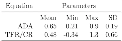
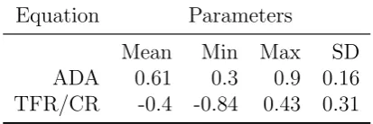
For the adaptive rule, we obtain similar results in the two treatments (see Tables 1 and 2). Interestingly, in the negative feedback treat-ment the majority of subject adopts a contrarian behavior, i.e. subjects form their predictions by assigning a negative coefficient to the observed trend. The extrapolative parameter of the TFR is equal to the average of all the estimated significant coefficients for the positive feedback treatment. We follow the same procedure for the negative feedback treatment to compute the parameter of the CR. In order to simulate the HSM, we use the following common specification:

α= 0.63, w= 0.44 and s=−0.44. Note that we decide not to implement exactly

the heuristics described in the original paper by Anufriev and Hommes (2012).

Table 1: Estimated parameter of the ADA rule and the TFR/CR rule for the positive feedback treatment. The mean is the average across significant coefficients.

Equation Parameters

Mean Min Max SD

ADA 0.65 0.21 0.9 0.19

TFR/CR 0.48 -0.34 1.3 0.66

5

Table 2: Estimated parameter of the ADA rule and the TFR/CR rule for the neg-ative feedback treatment. The mean is the average across significant coefficients.

Equation Parameters

Mean Min Max SD

ADA 0.61 0.3 0.9 0.16

TFR/CR -0.4 -0.84 0.43 0.31

3.1.2 EEA calibration

We can estimate the main parameters of the EEA algorithm, namelyφs,γ andφl,

for each subject using the maximum likelihood procedure. The two parameters related to the short-run predictions can be expressed in a close-form, while for

φl we rely on a numerical optimization. The probability distribution for one-step

ahead predictions of eq. (16) can be approximated by a Gaussian distribution, whose parameters can be expressed as:

iµt−1 =

pt−1+iφs ip e

t−1,t−1

(1 +iφs)

, (18)

σ2

i =

1

2γi (1 +iφs)

. (19)

The mean iµt−1 is determined the past prediction and past market price with

a given weight (φs). The variance is invariant over time and depends on the

given subject. By rearranging eq. (18), it is possible to express the mean of the distribution as a convex combination between past expectations and past market price:

iµt−1 = (1−αi)pt−1+αi ipet−1,t−1 , (20)

where the weight is given by αi =

iφs

1 +iφs

(note that iφs > −1). Estimating

iφs gives us information on how subjects adjust their short-run expectations over

time. According to the values for iφs, subjects combine in different ways past

predictions and prices. In particular, we identify the following behaviors: (i)

0<iφs <1 translates in 0 < αi <1/2 so that subjects try to adjust their future

predictions towards the market price; (ii) a value of iφs > 1 implies αi >

1

2 and,

as a consequence, subjects forecast values closed to previous predictions; (iii) for

negative values ofiφs subjects “overcorrect” their past expectations by submitting

predictions opposite to either market price −1

2 <iφs <0

or past predictions

−1

2 <iφs <−

1 3

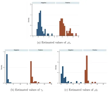
(panel a), ˆγi (panel b) and iφˆl (panel c) for both positive and negative feedback treatments.

In Table 3, we classify the subjects6

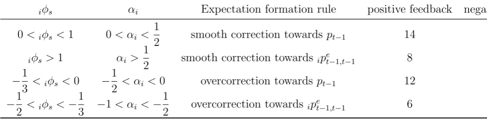
according to the above mentioned be-haviors. As can be seen, future predictions are computed differently depending on whether subjects participate in a positive or negative feedback treatment. In the positive feedback treatment, almost half of the subjects “overcorrect” their

forecasts (18 out of 40) either towards pt−1 or ip

e

t−1,t−1. In the negative feedback

treatment, the large majority of subjects (30 out of 44) adjust their predictions to be close to the market price. Interestingly, only a negligible minority (6 out of 44) take into account past expectations.

Table 3: Classification of subjects across the different expectation formation rules.

iφs αi Expectation formation rule positive feedback negativ

0<iφs <1 0< αi < 1

2 smooth correction towardspt−1 14

iφs >1 αi >

1

2 smooth correction towards ip

e

t−1,t−1 8

−1

3 <iφs <0 −

1

2 < αi <0 overcorrection towards pt−1 12

−1

2 <iφs <−

1

3 −1< αi <− 1

2 overcorrection towards ip

e

t−1,t−1 6

For the long-run expectations we estimate the individual values of iφl, common

for two, three and four-steps-ahead predictions of a given subject, and use the

value of γi obtained from short-run expectations. In order to simulate the EEA

we use the following set of parameters φs = 0.4, φl = 1.4 and γ = 0.4 for the

positive feedback treatment; φs = 0.15, φl = 1.4 and γ = 0.4 for the negative

feedback treatment. Note that those values are the median values of the estimated coefficients.

4

Simulation results

After a comprehensive description of the two algorithms, in this section we compare their performance in replicating the experimental results in markets with positive and negative feedback and for short- as well as long-run expectations.

6

We have eliminated the estimates of six subjects because of the estimated values ofiφs are

0

.5

1

1.5

-1 0 1 2 3 -1 0 1 2 3 Negative Positive

Density

(a) Estimated values ofiφs

0

.5

1

0 5 10 15 0 5 10 15 Negative Positive

Density

(b) Estimated values of γi

0

.2

.4

.6

0 5 10 15 0 5 10 15 Negative Positive

Density

(c) Estimated values ofiφl

Figure 7: Distribution of the estimated individual values for iφs, γi and iφl. Blue

4.1

Comparing the HSM and EEA to describe short-run

expectations

In order to simulate the HSM, in the first three periods we use the experimental

data to initiate the algorithm, assigning the same weight to each rule, i.e. nh,1 =

0.25,∀h. Starting from period three, we compute the fitness measure and the

weights nh,3 associated to each heuristic. For the subsequent periods we iterate

the algorithm detailed in the previous section.

In order to initiate the EEA algorithm, we use the experimental individual predictions and the first three realized prices, since the range of the action sets depends on the three past realized prices. Individual predictions are independent realizations from different distributions, so that we have six (the number of subjects in the group) different distributions and six predictions in every period and for every group. Once the short-term predictions are determined, we compute the market price by using either eq. (1) or eq. (2) according to the treatment the group belongs to.

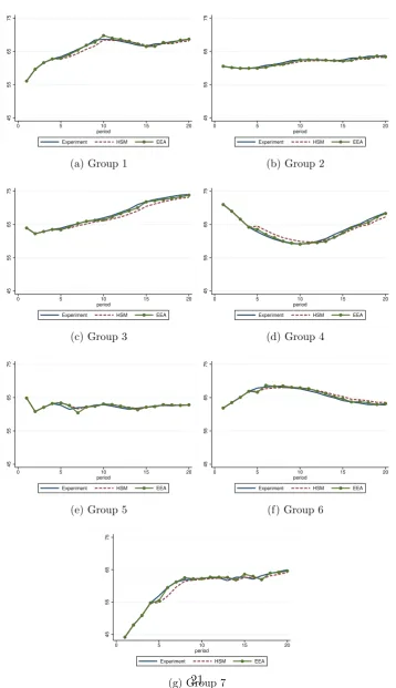
Figures 8 and 9 show the simulated market prices compared to the experimental market prices for all groups in positive and negative feedback treatment, respec-tively. From a preliminary inspection, both algorithms perform well in replicating experimental prices in the two treatments. Table 4 displays the values of the Mean Squared Error (MSE) for the two algorithms. The ability to foresight experimental prices is similar for both algorithms. Interestingly, we observe a systematic higher value of the MSE in the negative feedback treatment compared to the positive treatment. Thus, it seems that both algorithms are able to better capture the price time series in the positive than in the negative feedback treatment. This is in line with the literature on the application of the HSM in reproducing the experimental data.

45

55

65

75

0 5 10 15 20 period

Experiment HSM EEA

(a) Group 1

45

55

65

75

0 5 10 15 20 period

Experiment HSM EEA

(b) Group 2

45

55

65

75

0 5 10 15 20 period

Experiment HSM EEA

(c) Group 3

45

55

65

75

0 5 10 15 20 period

Experiment HSM EEA

(d) Group 4

45

55

65

75

0 5 10 15 20 period

Experiment HSM EEA

(e) Group 5

45

55

65

75

0 5 10 15 20 period

Experiment HSM EEA

(f) Group 6

45

55

65

75

0 5 10 15 20 period

Experiment HSM EEA

(g) Group 7

Figure 8: Simulation results based on the HSM and the EEA in the positive feedback treatment. The continuous black line is the experimental market price, the blue line is the market price generated using the HSM and the dashed grey

55

65

75

85

0 5 10 15 20 period

Experiment HSM EEA

(a) Group 1

55

65

75

85

0 5 10 15 20 period

Experiment HSM EEA

(b) Group 2

55

65

75

85

0 5 10 15 20 period

Experiment HSM EEA

(c) Group 3

55

65

75

85

0 5 10 15 20 period

Experiment HSM EEA

(d) Group 4

55

65

75

85

0 5 10 15 20 period

Experiment HSM EEA

(e) Group 5

55

65

75

85

0 5 10 15 20 period

Experiment HSM EEA

(f) Group 6

55

65

75

85

0 5 10 15 20 period

Experiment HSM EEA

(g) Group 7

55

65

75

85

0 5 10 15 20 period

Experiment HSM EEA

(h) Group 8

Figure 9: Simulation results based on the HSM and the EEA in the negative feedback treatment. The continuous black line is the experimental market price, the blue line is the market price generated using the HSM and the dashed grey

Table 4: Mean Squared Error of the HSM and EEA in describing the time series of experimental market prices.

Positive Negative

HSM EEA HSM EEA

Group 1 0.46 0.29 1.50 0.46

Group 2 0.22 0.06 0.97 3.21

Group 3 0.94 0.13 0.32 0.75

Group 4 0.99 0.13 2.00 1.84

Group 5 0.17 0.38 0.67 0.61

Group 6 0.48 0.16 2.16 1.77

Group 7 0.98 0.77 2.18 1.03

Group 8 - - 0.69 2.07

4.2

Comparing the HSM and EEA to describe long-run

expectations

One interesting contribution of the paper is the extension of the HSM in order to describe long-term expectations, with a simple linear extrapolative modification of the existing heuristics. The comparison with the EEA and its extension can give a rough idea of the goodness of the modified HSM in reproducing the long term-expectations. This is a relevant step to have a reliable framework to model long-term expectations in a realistic environment.

To the best of our knowledge, this is the first attempt in the literature on LtFEs to reproduce individual long-run expectations using the HSM. Despite the

fact that in the experiment subjects submit in each period t their expectations

for the remaining 20−t periods, we replicate the individual expectations up to

four steps ahead. Our choice represents a good compromise between considering the whole time-span and having a sufficient statistics to analyse the properties of the two algorithms as a function of the time horizon and comparing them to the experimental data.

We study the performance of the two algorithms in replicating the main statisti-cal properties of the experimental data, namely (i) the time series of the individual long-term expectations, (ii) the coordination of long-term predictions as a func-tion of the time horizon and (iii) the convergence of long-run expectafunc-tions to the fundamental value. It is worth mentioning that we do not have an aggregate vari-able as the market price for the long-run predictions, but just individual long-run predictions. When necessary, therefore, we rely on the average of the long-run expectations.

(across subjects) for 2, 3 and 4 steps ahead in the case of positive and negative feedback treatments. Once again, both algorithms seems to replicate the experi-mental data with a reasonable accuracy. Figures from 12 to 15 show the evolution of individual long run expectations in a representative group in the two treatments and for the two algorithms. A first glance, those figures shows that the individual long-run expectations generated by the two algorithms resemble the experimen-tal elicited expectations. In particular, we can observe in the positive feedback treatment, the cone-shape form of the predictions submitted in a given period as a function on the increasing time horizon. In the negative feedback treatment, we can observe the dynamical process of convergence to the REE of short- as well as long-run predictions.

In order to have a more quantitative comparison between the two algorithms, Tables 5 and 6 show the mean squared error of the simulated data (averaged over 100 Monte Carlo simulations) in describing the average long-run expectations. The EEA describes significantly better the long-run predictions than the modified HSM with the linear extrapolation heuristics.

In Figures 16 and 17, we compare the dynamical properties of the mutual coordination of long-run expectations and their convergence to the fundamental value. At a first inspection, it seems that the two algorithms are able to fairly well replicate the behavior of the experimental data, since the degree of coordination resulting from the simulated data is fairly close to the degree of coordination of experimental data. Additionally, the EEA and the HSM are capable of repro-ducing the more persistent heterogeneity observed for the long-run predictions as compared to the degree of coordination of the one-step-ahead predictions. A closer look at the behavior of the dispersion (measured with the MAD) of the long-run expectations as a function of the time horizon (panel (c) of Figure 16) shows that it increases linearly with the time horizon. This tendency is systematic in both, the negative and the positive feedback treatments. In the positive treatment, such lin-ear beahvior is similar to the empirical data. In the negative feedback treatment, instead, such increase of the dispersion over the horizons is much less evident, with some periods showing an absence of such a systematic increasing tendency.

Note that the HSM with the linear extrapolative trend for the long-run pre-dictions has built-in such characteristics. Any (linear) measure of dispersion of the predictions as a function of the time horizon will, therefore, exhibit a linear increase. This property is counter factual if we consider the negative feedback treatment. It is intuitive, in fact, that a simple linear extrapolation of prices can-not predict convergent prices to the fundamental value. Our numerical exercise, thus, shows that a the HSM should be modified with more complex heuristic rules to account for long-run expectations.

50

55

60

65

70

75

0 5 10 15 20

period

2step Exp 3step Exp 4step Exp Fundamental

(a) Group 1 - EXP

50

55

60

65

70

75

0 5 10 15 20

period

EEA 2step EEA 3step EEA 4step Fundamental

(b) Group 1 - EEA

50

55

60

65

70

75

0 5 10 15 20

period

HSM 2step HSM 3step HSM 4step Fundamental

(c) Group 1 - HSM

40

50

60

70

80

0 5 10 15 20

period

2step Exp 3step Exp 4step Exp Fundamental

(d) Group 4 - EXP

40

50

60

70

80

0 5 10 15 20

period

EEA 2step EEA 3step EEA 4step Fundamental

(e) Group 4 - EEA

40

50

60

70

80

0 5 10 15 20

period

HSM 2step HSM 3step HSM 4step Fundamental

(f) Group 4 - HSM

Figure 10: Average long-run expectations of two representative groups in the neg-ative feedback treatment for both experimental and simulated data. Blu, red and green lines represent the average 2, 3 and 4 step-ahead predictions, respectively.

2, 3 and 4 periods ahead. It shows that the degree of coordination resulting from the simulated data is fairly close to the degree of coordination of experimental data. Additionally, the EEA is able to reproduce the more persistent heterogeneity observed for the long-run predictions as compared to the degree of coordination of the one-step-ahead predictions.

5

EEA with the fundamental value as anchor

55

60

65

70

75

0 5 10 15 20

period

2step Exp 3step Exp 4step Exp Fundamental

(a) Group 1 - EXP

55

60

65

70

75

0 5 10 15 20

period

EEA 2step EEA 3step EEA 4step Fundamental

(b) Group 1 - EEA

55

60

65

70

75

0 5 10 15 20

period

HSM 2step HSM 3step HSM 4step Fundamental

(c) Group 1 - HSM

55

60

65

70

75

80

0 5 10 15 20

period

2step Exp 3step Exp 4step Exp Fundamental

(d) Group 4 - EXP

55

60

65

70

75

80

0 5 10 15 20

period

EEA 2step EEA 3step EEA 4step Fundamental

(e) Group 4 - EEA

60

65

70

75

80

0 5 10 15 20

period

HSM 2step HSM 3step HSM 4step Fundamental

(f) Group 4 - HSM

Figure 11: Average long run expectations of two representative groups in the pos-itive feedback treatment for both experimental and simulated data. Blu, red and green lines represent the average 2, 3 and 4 step-ahead predictions, respectively.

Table 5: Mean squared error of simulated long-run predictions in both positive and negative feedback treatments. We compute the average across groups quadratic distance between the average long-run experimental and EEA simulated predic-tions. Predictions are computed by using last observed price as an anchor.

Negative Positive

2step 3step 4step 2step 3step 4step

Group 1 2.46 5.16 4.97 0.23 0.59 1.21

Group 2 2.3 1.47 2.81 0.18 0.8 0.94

Group 3 0.3 2.88 3.66 0.26 0.5 1.07

Group 4 1.87 1.17 3.88 0.13 0.55 3.02

Group 5 0.89 0.77 0.93 0.38 0.52 1.18

Group 6 5.41 1.67 22.94 0.2 0.5 1.15

Group 7 2.06 1.31 2.06 1.03 2.37 5.23

-0 20 40 60 80 100

0 5 10 15 20 Period

(a) Period 5 -EXP 0 20 40 60 80 100

0 5 10 15 20 Period

(b) Period 5 -EEA 0 20 40 60 80 100

0 5 10 15 20 Period

(c) Period 5 -HSM 0 20 40 60 80 100

0 5 10 15 20 Period

(d) Period 6 -EXP 0 20 40 60 80 100

0 5 10 15 20 Period

(e) Period 6 - EEA

0 20 40 60 80 100

0 5 10 15 20 Period

(f) Period 6 -HSM 0 20 40 60 80 100

0 5 10 15 20 Period

(g) Period 7 -EXP 0 20 40 60 80 100

0 5 10 15 20 Period

(h) Period 7 -EEA 0 20 40 60 80 100

0 5 10 15 20 Period

(i) Period 7 - HSM

0 20 40 60 80 100

0 5 10 15 20 Period

(j) Period 8 - EXP

0 20 40 60 80 100

0 5 10 15 20 Period

(k) Period 8 -EEA 0 20 40 60 80 100

0 5 10 15 20 Period

(l) Period 8 - HSM

0 20 40 60 80 100

0 5 10 15 20 Period

(m) Period 9 -EXP 0 20 40 60 80 100

0 5 10 15 20 Period

(n) Period 9 -EEA 0 20 40 60 80 100

0 5 10 15 20 Period

(o) Period 9 -HSM 0 20 40 60 80 100

0 5 10 15 20 Period

(p) Period 10 -EXP 0 20 40 60 80 100

0 5 10 15 20 Period

(q) Period 10 -EEA 0 20 40 60 80 100

0 5 10 15 20 Period

(r) Period 10 -HSM

Figure 12: Individual long-run predictions both real and simulated of Group 1 of the negative feedback treatment from period 5 to period 10. The black dots are

0 20 40 60 80 100

0 5 10 15 20 Period

(a) Period 11 -EXP 0 20 40 60 80 100

0 5 10 15 20 Period

(b) Period 11 -EEA 0 20 40 60 80 100

0 5 10 15 20 Period

(c) Period 11 -HSM 0 20 40 60 80 100

0 5 10 15 20 Period

(d) Period 12 -EXP 0 20 40 60 80 100

0 5 10 15 20 Period

(e) Period 12 -EEA 0 20 40 60 80 100

0 5 10 15 20 Period

(f) Period 12 -HSM 0 20 40 60 80 100

0 5 10 15 20 Period

(g) Period 13 -EXP 0 20 40 60 80 100

0 5 10 15 20 Period

(h) Period 13 -EEA 0 20 40 60 80 100

0 5 10 15 20 Period

(i) Period 13 -HSM 0 20 40 60 80 100

0 5 10 15 20 Period

(j) Period 14 -EXP 0 20 40 60 80 100

0 5 10 15 20 Period

(k) Period 14 -EEA 0 20 40 60 80 100

0 5 10 15 20 Period

(l) Period 14 -HSM 0 20 40 60 80 100

0 5 10 15 20 Period

(m) Period 15 -EXP 0 20 40 60 80 100

0 5 10 15 20 Period

(n) Period 15 -EEA 0 20 40 60 80 100

0 5 10 15 20 Period

(o) Period 15 -HSM

0 20 40 60 80 100

0 5 10 15 20 Period

(a) Period 5 -EXP 0 20 40 60 80 100

0 5 10 15 20 Period

(b) Period 5 -EEA 0 20 40 60 80 100

0 5 10 15 20 Period

(c) Period 5 -HSM 0 20 40 60 80 100

0 5 10 15 20 Period

(d) Period 6 -EXP 0 20 40 60 80 100

0 5 10 15 20 Period

(e) Period 6 - EEA

0 20 40 60 80 100

0 5 10 15 20 Period

(f) Period 6 -HSM 0 20 40 60 80 100

0 5 10 15 20 Period

(g) Period 7 -EXP 0 20 40 60 80 100

0 5 10 15 20 Period

(h) Period 7 -EEA 0 20 40 60 80 100

0 5 10 15 20 Period

(i) Period 7 - HSM

0 20 40 60 80 100

0 5 10 15 20 Period

(j) Period 8 - EXP

0 20 40 60 80 100

0 5 10 15 20 Period

(k) Period 8 -EEA 0 20 40 60 80 100

0 5 10 15 20 Period

(l) Period 8 - HSM

0 20 40 60 80 100

0 5 10 15 20 Period

(m) Period 9 -EXP 0 20 40 60 80 100

0 5 10 15 20 Period

(n) Period 9 -EEA 0 20 40 60 80 100

0 5 10 15 20 Period

(o) Period 9 -HSM 0 20 40 60 80 100

0 5 10 15 20 Period

(p) Period 10 -EXP 0 20 40 60 80 100

0 5 10 15 20 Period

(q) Period 10 -EEA 0 20 40 60 80 100

0 5 10 15 20 Period

(r) Period 10 -HSM

Figure 14: Individual long-run predictions both real and simulated of Group 1 of the positive feedback treatment from period 5 to period 10. The black dots are

0 20 40 60 80 100

0 5 10 15 20 Period

(a) Period 11 -EXP 0 20 40 60 80 100

0 5 10 15 20 Period

(b) Period 11 -EEA 0 20 40 60 80 100

0 5 10 15 20 Period

(c) Period 11 -HSM 0 20 40 60 80 100

0 5 10 15 20 Period

(d) Period 12 -EXP 0 20 40 60 80 100

0 5 10 15 20 Period

(e) Period 12 -EEA 0 20 40 60 80 100

0 5 10 15 20 Period

(f) Period 12 -HSM 0 20 40 60 80 100

0 5 10 15 20 Period

(g) Period 13 -EXP 0 20 40 60 80 100

0 5 10 15 20 Period

(h) Period 13 -EEA 0 20 40 60 80 100

0 5 10 15 20 Period

(i) Period 13 -HSM 0 20 40 60 80 100

0 5 10 15 20 Period

(j) Period 14 -EXP 0 20 40 60 80 100

0 5 10 15 20 Period

(k) Period 14 -EEA 0 20 40 60 80 100

0 5 10 15 20 Period

(l) Period 14 -HSM 0 20 40 60 80 100

0 5 10 15 20 Period

(m) Period 15 -EXP 0 20 40 60 80 100

0 5 10 15 20 Period

(n) Period 15 -EEA 0 20 40 60 80 100

0 5 10 15 20 Period

(o) Period 15 -HSM

0

2

4

6

8

10

Negative Positive

1 2 3 4 5 6 7 8 9 1011121314151617181920 1 2 3 4 5 6 7 8 9 1011121314151617181920

MADc 1step MADc 2step MADc 3step MADc 4step

(a) Experimental

0

2

4

6

8

10

N P

1 2 3 4 5 6 7 8 9 1011121314151617181920 1 2 3 4 5 6 7 8 9 1011121314151617181920

MADc 1step EEA MADc 2step EEA MADc 3step EEA MADc 4step EEA

(b) Simulated

0

5

10

15

20

1 2 3 4 5 6 7 8 9 1011121314151617181920 1 2 3 4 5 6 7 8 9 1011121314151617181920

Negative Positive

MADc 1step HSM MADc 2step HSM MADc 3step HSM MADc step HSM

(c) Simulated

0

5

10

15

20

Negative Positive

1 2 3 4 5 6 7 8 9 1011121314151617181920 1 2 3 4 5 6 7 8 9 1011121314151617181920

MAD 1step MAD 2step MAD 3step MAD 4step

(a) Experimental

0

5

10

15

20

Negative Positive

1 2 3 4 5 6 7 8 9 1011121314151617181920 1 2 3 4 5 6 7 8 9 1011121314151617181920

MAD 1step EEA MAD 2step EEA MAD 3step EEA MAD 4step EEA

(b) Simulated EEA

0

5

10

15

20

Negative Positive

1 2 3 4 5 6 7 8 9 1011121314151617181920 1 2 3 4 5 6 7 8 9 1011121314151617181920

MAD 1step HSM MAD 2step HSM MAD 3step HSM MAD 4step HSM

(c) Simulated HSM

Table 6: Mean squared error of simulated long-run predictions in both positive and negative feedback treatments. We compute the average (across groups) quadratic distance between the average long-run experimental and HSM simulated predic-tions.

Negative Positive

2step 3step 4step 2step 3step 4step

Group 1 3.78 9.39 12.31 1.40 2.68 4.51

Group 2 2.42 10.09 13.35 0.05 0.59 0.25

Group 3 2.92 4.87 9.01 0.51 1.01 1.96

Group 4 4.69 7.90 9.08 1.20 2.71 3.95

Group 5 0.59 0.56 0.35 0.29 0.42 0.79

Group 6 10.48 19.64 34.03 1.14 2.37 3.66

Group 7 0.81 1.37 1.76 1.94 2.26 2.19

Group 8 3.05 6.41 6.97 - -

-market price. Instead, in Model (2) we use as explanatory variables past indi-vidual short-run expectations and the fundamental value. Our results show that, whereas Model (1) performs well in the two feedback mechanism showing the rele-vance of past prices in the formation of expectations, Model (2) clearly highlights the pivotal role of the fundamental value in determining short-run expectations in negative feedback markets with a coefficient close to 1, compared to the role of the fundamental price in the formation of short-run expectations in markets with

positive feedback (with a coefficient of 0.09).

Table 7: Dynamic panel regression of individual short-run expectations. Depen-dent variable: individual short-run expectations. Standard errors in parentheses.

Positive Negative

Model(1) Model(2) Model(1) Model(2)

pt−1 0.77∗∗∗ (0.05) 0.70∗∗∗ (0.02)

ipet−1,t−1 0.23∗∗∗ (0.05) 0.30∗∗∗ (0.02)

pf 0.09∗ _{(0.05) 0.99}∗∗∗ _(0.04)

ipet−1,t−1 0.91

∗∗∗ _{(0.06) 0.01 (0.04)}

N 798 798 912 912

Waldχ2

134952.46∗∗∗ _32720.83∗∗∗ _15010.52∗∗∗ _15494.63∗∗∗

choice of the right anchor is therefore crucial. Colasante et al. (2018c) show that, using the market price as anchor in markets with positive feedback, they obtain a fairly good replication of the subjects’ expectations elicited in the laboratory experiment. In this work, they also compare the performance of the EEA with an

alternative model like the so-called noisy rational expectations, that is based on

the idea that subjects have homogeneous rational expectations.7

They conclude that this model provides a good approximation of the expectations elicited in the negative feedback treatment. However, even though (experimental) predictions in markets with negative feedback quickly converge to the fundamental value, they observe a persistent heterogeneity of expectations in the experimental data that is not found in the simulated expectations.

In order to reproduce the main features typically observed in (experimental) subjects’ expectations concerning heterogeneity and convergence of long-run ex-pectations, we implement an alternative version of the EEA, where we use the

fundamental value as anchor.8

We compute then agents’ individual predictions

for different forecast horizons k, where k = 1,2,3, using the fundamental value

(instead of past market prices) as anchor. In other words, the fitness measure is computed using eqs. (14) and (15) considering instead the fundamental value as a reference point as follows:

iVj,t˜ = (pf −iajt)

2

+φs (ipet−1,t−1−iajt)

2

, (21)

iV˜j,tk =|pf −iakjt|+φl |ipet−k−1,t−1−iakjt|. (22)

Settingφ 6= 0 we are able to obtain heterogeneous predictions as a result of past

individual expectations. In order to illustrate our results, Figures 19 and 18 show as an example the average of individual predictions two, three and four steps ahead in two representative groups in market with positive and negative feedback. Table 8 displays the MSE comparing the experimental data and the simulated expectations in markets with positive and negative feedback. The results obtained show that the EEA with the fundamental value as anchor performs better to replicate, on average, the experimental data in the markets with negative feedback compare to its performance in the markets with positive feedback.

With these results we provide further evidence that subjects form their ex-pectations following different rules depending on the feedback system. In markets

7

In the EEA homogeneous rational expectations are implemented by setting the mean of the probability distribution of each agent (i.e, iµ) equal to the fundamental value in the centre of

the range of actions. They then setφ= 0 and replacept−1 with the fundamental value

8

50

55

60

65

70

75

0 5 10 15 20 period

2step Exp 3step Exp 4step Exp Fundamental

(a) Group 1

50

55

60

65

70

75

0 5 10 15 20 period

EEA_R 2step EEA_R 3step EEA_R 4step Fundamental

(b) Group 1

60

65

70

0 5 10 15 20 period

2step Exp 3step Exp 4step Exp Fundamental

(c) Group 4

60

65

70

0 5 10 15 20 period

EEA_R 2step EEA_R 3step EEA_R 4step Fundamental

(d) Group 4

Figure 18: Average long run expectations in the negative feedback treatment.

with negative feedback, subjects’ expectations are mainly driven by the fundamen-tal value, while in the positive feedback system the reference point is the market price.

6

Conclusion

55

60

65

70

75

0 5 10 15 20 period

2step Exp 3step Exp 4step Exp Fundamental

(a) Group 1

55

60

65

70

75

0 5 10 15 20 period

2step EEA 3step EEA 4step EEA Fundamental

(b) Group 1

55

60

65

70

75

80

0 5 10 15 20 period

2step Exp 3step Exp 4step Exp Fundamental

(c) Group 4

60

65

70

75

80

0 5 10 15 20 period

2step EEA 3step EEA 4step EEA Fundamental

(d) Group 4

Figure 19: Average long run expectations in the positive feedback treatment.

Table 8: Mean squared error of simulated long run predictions in both positive and negative feedback treatments. We compute the quadratic distance between the average experimental and EEA simulated predictions. Predictions are computed by using fundamental value as an anchor.

Negative Positive

2step 3step 4step 2step 3step 4step

Group 1 0.84 1.21 1.8 6.86 7.50 8.34

Group 2 0.48 0.61 0.7 29.30 74.54 69.84

Group 3 0.23 0.6 1.62 11.11 28.08 30.28

Group 4 3.59 3.61 5.33 8.71 25.33 28.59

Group 5 0.17 0.23 1.15 4.08 6.62 6.74

Group 6 0.65 0.97 0.73 3.07 8.62 11.65

Group 7 0.8 1.33 1.12 18.85 17.35 17.10

-“non-parametric”, so that the predictions are chosen according to a specific prob-ability distribution. The two algorithms are based on the common principle of anchor and adjustment rule. Regarding short run predictions, we observe that both algorithms perform well in replicating individual predictions. In order to simulate long-run predictions, we have introduced a straightforward extension of the HSM: a linear extrapolation of short-run predictions across different horizons. A considerable difference emerges between the two algorithms: the linear extrap-olation provide a good approximation of the main stylized facts in the positive feedback treatment. In the negative feedback system, the coordination and con-vergence properties are better explained by the EEA. Moreover, we have performed an exercise to test whether a change in the anchor can lead to better results in replicating the experimental data. We have considered as an alternative anchor the fundamental value instead of the market price. This modification leads to better simulation results in the negative feedback system, while in the positive feedback market we obtain a worse performance. The comparison between such different algorithms helps us to understand that the subjects form their expecta-tions using different anchors. The EEA is a good and flexible tool to replicate short and long-run predictions in both positive and negative feedback systems. The linear extrapolation we have implemented in this paper as en extension of the HSM to compute long-run expectations is not sufficiently flexible to capture the behavior in the different feedback environments: a more complex structure is needed to replicate the properties of long-run predictions, which is the focus of future research.

Acknowledgement

References

Mikhail Anufriev and Cars Hommes. Evolutionary selection of individual

expecta-tions and aggregate outcomes in asset pricing experiments. American Economic

Journal: Microeconomics, 4(4):35–64, 2012.

Mikhail Anufriev, Cars Assenza, Tiziana and, and Domenico Massaro. Inter-est rate rules and macroeconomic stability under heterogeneous expectations.

Macroeconomic Dynamics, 17(08):1574–1604, 2013.

Tiziana Assenza, Peter Heemeijer, Cars Hommes, and Domenica Massaro. In-dividual Expectations and Aggregate Macro Behavior. Dnb working papers, Netherlands Central Bank, Research Department, May 2011.

Tiziana Assenza, Te Bao, Cars Hommes, and Domenico Massaro. Experiments

on expectations in macroeconomics and finance. In Experiments in

macroeco-nomics, pages 11–70. Emerald Group Publishing Limited, 2014.

Te Bao and Li Ding. Nonrecourse mortgage and housing price boom, bust, and

rebound. Real Estate Economics, 44(3):584–605, 2016.

Te Bao, Cars Hommes, Joep Sonnemans, and Jan Tuinstra. Individual

expecta-tions, limited rationality and aggregate outcomes. Journal of Economic

Dynam-ics and Control, 36(8):1101–1120, 2012.

Te Bao, John Duffy, and Cars Hommes. Learning, forecasting and optimizing: An

experimental study. European Economic Review, 61:186–204, 2013.

William A Brock and Cars H Hommes. Heterogeneous beliefs and routes to chaos

in a simple asset pricing model. Journal of Economic dynamics and Control, 22

(8-9):1235–1274, 1998.

Annarita Colasante, Simone Alfarano, Eva Camacho, and Mauro Gallegati.

Long-run expectations in a learning-to-forecast experiment. Applied Economics

Let-ters, 25(10):681–687, 2018a.

Annarita Colasante, Simone Alfarano, and Eva Camacho-Cuena. The term struc-ture of cross-sectional dispersion of expectations in a Learning-to-Forecast Ex-periment. Technical report, 2018b.

Annarita Colasante, Simone Alfarano, Eva Camacho-Cuena, and Mauro Gallegati. Long-run expectations in a Learning-to-Forecast Experiment: A Simulation

Ap-proach. Journal of Evolutionary Economics, 2018c. doi:

Camille Cornand and Cheick Kader M’baye. Does inflation targeting matter? an

experimental investigation. Macroeconomic Dynamics, pages 1–40, 2016.

Cees Diks and Roy Van Der Weide. Herding, a-synchronous updating and

hetero-geneity in memory in a cbs. Journal of Economic Dynamics and Control, 29(4):

741–763, 2005.

Milton Friedman. Essays in Positive Economics. University of Chicago Press,

1966.

Peter Heemeijer, Cars Hommes, Joep Sonnemans, and Jan Tuinstra. Price stability and volatility in markets with positive and negative expectations feedback: An

experimental investigation. Journal of Economic Dynamics and Control, 33(5):

1052–1072, 2009.

Cars Hommes. Behavioral rationality and heterogeneous expectations in complex

economic systems. Cambridge University Press, 2013.

Cars Hommes. Behavioral & experimental macroeconomics and policy analysis: a complex systems approach. Working paper series, European Central Bank, November 2018.

Cars Hommes and Thomas Lux. Individual expectations and aggregate behavior

in learning-to-forecast experiments. Macroeconomic Dynamics, 17(02):373–401,

2013.

Cars Hommes, Joep Sonnemans, Jan Tuinstra, and Henk van de Velden. A

strat-egy experiment in dynamic asset pricing. Journal of Economic Dynamics and

Control, 29(4):823–843, 2005.

Daniel Kahneman and Amos Tversky. On the psychology of prediction.

Psycho-logical Review, 80(4):237, 1973.

Robert E Lucas Jr and Edward C Prescott. Investment under uncertainty.

Econo-metrica: Journal of the Econometric Society, pages 659–681, 1971.

Ramon Marimon, Stephen E Spear, and Shyam Sunder. Expectationally driven

market volatility: an experimental study. Journal of Economic Theory, 61(1):

74–103, 1993.

John F Muth. Rational expectations and the theory of price movements.

Econo-metrica: Journal of the Econometric Society, pages 315–335, 1961.

Herbert Alexander Simon. Models of man: social and rational; mathematical

The instructions and the scree-shot are not intended to be published. We include this information for the convenience of the referees.

A

Instructions and Screenshot

[General instructions]

Welcome to the Laboratory of Experimental Economics! You are participating in an experiment in which you will take decisions in a financial market. The instructions are very simple but, please, read them carefully.

During the whole experiment you will play with experimental currency unit (ECU) and, at the end of the experiment, your final profit, summed to the 3? for the show-up fee, will be converted in Euro according to the following exchange

rate: 1 Euro=500 ECU. The total amount will be paid at the end of the

exper-iment by cash.

[Only in the positive feedback treatment]

You are a financial advisor to a pension fund that wants to invest an amount of money to buy an asset. The pension fund will allocate its money between a bank account which pays fix interest rate and a risky asset that pays dividends. The allocation depends on your forecast on the evolution of the asset price. When making your predictions remember that the asset price each period is affected: positively by the dividend, negatively by the interest rate and positively by the investors’ expectations on the asset price in that period.

Your task is to predict the price for 20 periods. In each period (t) you will

predict the price for all the remaining 20−t periods, that is, in period 1 you will

submit 20 predictions starting from the prediction about the price at the end of period 1, in period 2 you will submit 19 predictions and so on. Your predictions must be between 0 and 100.