Learning Grounded Meaning Representations with Autoencoders
Carina SilbererandMirella Lapata
Institute for Language, Cognition and Computation School of Informatics, University of Edinburgh
10 Crichton Street, Edinburgh EH8 9AB
[email protected],[email protected]
Abstract
In this paper we address the problem of grounding distributional representations of lexical meaning. We introduce a new model which uses stacked autoencoders to learn higher-level embeddings from tex-tual and visual input. The two modali-ties are encoded as vectors of attributes and are obtained automatically from text and images, respectively. We evaluate our model on its ability to simulate similar-ity judgments and concept categorization. On both tasks, our approach outperforms baselines and related models.
1 Introduction
Recent years have seen a surge of interest in sin-gle word vector spaces (Turney and Pantel, 2010; Collobert et al., 2011; Mikolov et al., 2013) and their successful use in many natural language ap-plications. Examples include information retrieval (Manning et al., 2008), search query expansions (Jones et al., 2006), document classification (Se-bastiani, 2002), and question answering (Yih et al., 2013). Vector spaces have been also popular in cognitive science figuring prominently in simula-tions of human behavior involving semantic prim-ing, deep dyslexia, text comprehension, synonym selection, and similarity judgments (see Griffiths et al., 2007). In general, these models specify mechanisms for constructing semantic representa-tions from text corpora based on thedistributional hypothesis (Harris, 1970): words that appear in similar linguistic contexts are likely to have related meanings.
Word meaning, however, is also tied to the physical world. Words aregrounded in the exter-nal environment and relate to sensorimotor experi-ence (Regier, 1996; Landau et al., 1998; Barsalou, 2008). To account for this, new types of perceptu-ally grounded distributional models have emerged.
These models learn the meaning of words based on textual and perceptual input. The latter is ap-proximated by feature norms elicited from humans (Andrews et al., 2009; Steyvers, 2010; Silberer and Lapata, 2012), visual information extracted automatically from images, (Feng and Lapata, 2010; Bruni et al., 2012a; Silberer et al., 2013) or a combination of both (Roller and Schulte im Walde, 2013). Despite differences in formulation, most existing models conceptualize the problem of meaning representation as one of learning from multiple views corresponding to different modali-ties. These models still represent words as vectors resulting from the combination of representations with different statistical properties that do not nec-essarily have a natural correspondence (e.g., text and images).
In this work, we introduce a model, illus-trated in Figure 1, which learns grounded mean-ing representations by mappmean-ing words and im-ages into a common embedding space. Our model uses stacked autoencoders (Bengio et al., 2007) to induce semantic representations integrating vi-sual and textual information. The literature de-scribes several successful approaches to multi-modal learning using different variants of deep networks (Ngiam et al., 2011; Srivastava and Salakhutdinov, 2012) and data sources including text, images, audio, and video. Unlike most pre-vious work, our model is defined at a finer level of granularity — it computes meaning representa-tions forindividualwords and is unique in its use ofattributesas a means of representing the textual and visual modalities. We follow Silberer et al. (2013) in arguing that an attribute-centric repre-sentation is expedient for several reasons.
Firstly, attributes provide a natural way of ex-pressing salient properties of word meaning as demonstrated in norming studies (e.g., McRae et al., 2005) where humans often employ attributes when asked to describe a concept. Secondly, from
a modeling perspective, attributes allow for eas-ier integration of different modalities, since these are rendered in the same medium, namely, lan-guage. Thirdly, attributes are well-suited to de-scribing visual phenomena (e.g., objects, scenes, actions). They allow to generalize to new in-stances for which there are no training exam-ples available and to transcend category and task boundaries whilst offering a generic description of visual data (Farhadi et al., 2009).
Our model learns multimodal representations from attributes which are automatically inferred from text and images. We evaluate the embed-dings it produces on two tasks, namely word sim-ilarity and categorization. In the first task, model estimates of word similarity (e.g.,gem–jewel are similar butglass–magician are not) are compared against elicited similarity ratings. We performed a large-scale evaluation on a new dataset consist-ing of human similarity judgments for 7,576 word pairs. Unlike previous efforts such as the widely used WordSim353 collection (Finkelstein et al., 2002), our dataset contains ratings for visual and textual similarity, thus allowing to study the two modalities (and their contribution to meaning rep-resentation) together and in isolation. We also assess whether the learnt representations are ap-propriate for categorization, i.e., grouping a set of objects into meaningful semantic categories (e.g., peach and apple are members of FRUIT,
whereaschairandtableareFURNITURE). On both
tasks, our model outperforms baselines and related models.
2 Related Work
The presented model has connections to several lines of work in NLP, computer vision research, and more generally multimodal learning. We re-view related work in these areas below.
Grounded Semantic Spaces Grounded seman-tic spaces are essentially distributional models augmented with perceptual information. A model akin to Latent Semantic Analysis (Landauer and Dumais, 1997) is proposed in Bruni et al. (2012b) who concatenate two independently constructed textual and visual spaces and subsequently project them onto a lower-dimensional space using Singu-lar Value Decomposition.
Several other models have been extensions of Latent Dirichlet Allocation (Blei et al., 2003) where topic distributions are learned from words
and other perceptual units. Feng and Lapata (2010) use visual words which they extract from a corpus of multimodal documents (i.e., BBC news articles and their associated images), whereas oth-ers (Steyvoth-ers, 2010; Andrews et al., 2009; Silberer and Lapata, 2012) use feature norms obtained in longitudinal elicitation studies (see McRae et al. (2005) for an example) as an approximation of the visual environment. More recently, topic mod-els which combine both feature norms and vi-sual words have also been introduced (Roller and Schulte im Walde, 2013). Drawing inspiration from the successful application of attribute clas-sifiers in object recognition, Silberer et al. (2013) show that automatically predicted visual attributes act as substitutes for feature norms without any critical information loss.
The visual and textual modalities on which our model is trained are decoupled in that they are not derived from the same corpus (we would expect co-occurring images and text to correlate to some extent) but unified in their representation by natu-ral language attributes. The use of stacked autoen-coders to extract a shared lexical meaning repre-sentation is new to our knowledge, although, as we explain below related to a large body of work on deep learning.
Multimodal Deep Learning Our work employs deep learning (a.k.a deep networks) to project lin-guistic and visual information onto a unified rep-resentation that fuses the two modalities together. The goal of deep learning is to learn multiple lev-els of representations through a hierarchy of net-work architectures, where higher-level representa-tions are expected to help define higher-level con-cepts.
so as to infer some missing modality from others (e.g., to infer text from images and vice versa); in contrast, we aim to learn an optimal representa-tion for each modality and their optimal combi-nation. Secondly, our problem setting is different from the former studies, which usually deal with classification tasks and fine-tune the deep neural networks using training data with explicit class la-bels; in contrast we fine-tune our autoencoders us-ing a semi-supervised criterion. That is, we use indirect supervision in the form of object classifi-cation in addition to the objective of reconstruct-ing the attribute-centric input representation. 3 Autoencoders for Grounded Semantics
3.1 Background
Our model learns higher-level meaning represen-tations for single words from textual and visual input in a joint fashion. We first briefly review autoencoders in Section 3.1 with emphasis on as-pects relevant to our model which we then de-scribe in Section 3.2.
Autoencoders An autoencoder is an unsuper-vised neural network which is trained to recon-struct a given input from its latent representation (Bengio, 2009). It consists of an encoder fθwhich maps an input vector x(i) to a latent representa-tion y(i)= f
θ(x(i)) =s(Wx(i)+b), with s being a non-linear activation function, such as a sig-moid function. A decodergθ0 then aims to recon-struct input x(i) from y(i), i.e., ˆx(i)=g
θ0(y(i)) =
s(W0y(i)+b0). The training objective is the de-termination of parameters ˆθ={W,b} and ˆθ0 = {W0,b0}that minimize the average reconstruction error over a set of input vectors{x(1),...,x(n)}:
ˆ
θ,θˆ0=argmin θ,θ0
1
n
n
∑
i=1L(x
(i),g
θ0(fθ(x(i)))), (1)
whereLis a loss function, such as cross-entropy. Parametersθandθ0can be optimized by gradient descent methods.
Autoencoders are a means to learn representa-tions of some input by retaining useful features in the encoding phase which help to reconstruct the input, whilst discarding useless or noisy ones. To this end, different strategies have been employed to guide parameter learning and constrain the hid-den representation. Examples include imposing a bottleneck to produce an under-complete rep-resentation of the input, using sparse representa-tions, ordenoising.
Denoising Autoencoders The training criterion with denoising autoencoders is the reconstruction of clean input x(i) given a corrupted version ˜x(i) (Vincent et al., 2010). The underlying idea is that the learned latent representation is good if the au-toencoder is capable of reconstructing the actual input from its corruption. The reconstruction error for an inputx(i)with loss functionLthen is:
L(x(i),gθ0(fθ(˜x(i)))) (2)
One possible corruption process ismasking noise, where the corrupted version ˜x(i) results from ran-domly setting a fractionvofx(i)to 0.
Stacked Autoencoders Several (denoising) au-toencoders can be used as building blocks to form a deep neural network (Bengio et al., 2007; Vin-cent et al., 2010). For that purpose, the autoen-coders are pre-trained layer by layer, with the cur-rent layer being fed the latent representation of the previous autoencoder as input. Using this unsuper-vised pre-training procedure, initial parameters are found which approximate a good solution. Subse-quently, the original input layer and hidden repre-sentations of all the autoencoders are stacked and all network parameters are fine-tuned with back-propagation.
To further optimize the parameters of the net-work, a supervised criterion can be imposed on top of the last hidden layer such as the minimization of a prediction error on a supervised task (Bengio, 2009). Another approach is to unfold the stacked autoencoders and fine-tune them with respect to the minimization of the global reconstruction error (Hinton and Salakhutdinov, 2006). Alternatively, a semi-supervised criterion can be used (Ranzato and Szummer, 2008; Socher et al., 2011) through combination of the unsupervised training criterion (global reconstruction) with a supervised criterion (prediction of some target given the latent repre-sentation).
3.2 Semantic Representations
... ... ...
inputx
TEXT
W(1)
W(3)
... ... ...
IMAGES
W(2)
W(4)
... bimodal coding˘y
W(50)
W(5)
... softmaxˆt
W(6) ...
...
W(30)
... ...
W(40)
... reconstructionxˆ
W(10)
...
[image:4.595.131.475.61.256.2]W(20)
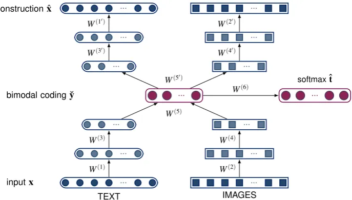
Figure 1: Stacked autoencoder trained with semi-supervised objective. Input to the model are single-word vector representations obtained from text and images. Vector dimensions correspond to textual and visual attributes, respectively (see Table 1).
in Section 4.1. We first train SAEs with two hid-den layers (codings) for each modality separately. Then, we join these two SAEs by feeding their re-spective second coding simultaneously to another autoencoder, whose hidden layer thus yields the fused meaning representation. Finally, we stack all layers and unfold them in order to fine-tune the SAE. Figure 1 illustrates the model.
Unimodal Autoencoders For both modalities, we use the hyperbolic tangent function as activa-tion funcactiva-tion for encoderfθand decodergθ0and an entropic loss function forL. The weights of each autoencoder are tied, i.e.,W0=WT. We employ
denoising autoencoders (DAEs) for pre-training the textual modality. Regarding the visual autoen-coder, we derive a new (‘denoised’) target vector to be reconstructed for each input vectorx(i), and treat x(i) itself as corrupted input. The unimodal autoencoder is thus trained to denoise a given in-put. The target vector is derived as follows: each objectoin our data is represented by multiple im-ages, and each image is in turn represented by a visual attribute vectorx(i). The target vector is the sum ofx(i) and the centroidx(j)of the remaining attribute vectors representing objecto.
Bimodal Autoencoder The bimodal autoen-coder is fed with the concatenated final hidden codings of the visual and textual modalities as in-put and maps these inin-puts to a joint hidden layer ˘y withB units. We normalize both unimodal input
codings to unit length. Again, we use tied weights for the bimodal autoencoder. We also encourage the autoencoder to detect dependencies between the two modalities while learning the mapping to the bimodal hidden layer. We therefore apply masking noise to one modality with a masking fac-torv(see Section 3.1), so that the corrupted modal-ity optimally has to rely on the other modalmodal-ity in order to reconstruct its missing input features. Stacked Bimodal Autoencoder We finally build a stacked bimodal autoencoder (SAE) with all ptrained layers and fine-tune them with re-spect to a semi-supervised criterion. That is, we unfold the stacked autoencoder and furthermore add a softmax output layer on top of the bimodal layer ˘y that outputs predictions ˆt with respect to the inputs’ object labels (e.g.,boat):
ˆt(i)= exp(W(6)˘y(i)+b(6))
∑Ok=1exp(Wk(6.)˘y(i)+b(6)
k )
, (3)
with weightsW(6)∈RO×B,b(6)∈RO×1, whereO
is the number of unique object labels. The over-all objective to be minimized is therefore the weighted sum of the reconstruction error Lr and
the classification errorLc:
L=1n
∑
ni=1
δrLr(x(i),ˆx(i))+δcLc(t(i),ˆt(i))
+λR (4)
where δr and δc are weighting parameters that
eats seeds has beak has claws has handlebar has wheels has wings is yellow made of wood
canary 0.05 0.24 0.15 0.00 –0.10 0.19 0.34 0.00
V
isual
trolley 0.00 0.00 0.00 0.30 0.32 0.00 0.00 0.25 bird:n breed:v cage:n chirp:v fly:v track:n ride:v run:v rail:n wheel:n
canary 0.16 0.19 0.39 0.13 0.13 0.00 0.00 0.00 0.00 –0.05
Te
xtual
[image:5.595.93.503.70.150.2]trolley –0.40 0.00 0.00 0.00 0.00 0.14 0.16 0.33 0.17 0.20
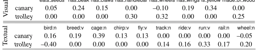
Table 1: Examples of attribute-based representations provided as input to our autoencoders.
Lc and Lr are entropic loss functions, and R is
a regularization term with R=∑5j=12||W(j)||2+
||W(6)||2. Finally,ˆt(i)is the object label vector pre-dicted by the softmax layer for input vector x(i), andt(i)is the correct object label, represented as a
O-dimensional one-hot vector1.
The additional supervised criterion drives the learning towards a representation capable of dis-criminating between different objects. Further-more, the semi-supervised setting affords flexibil-ity, allowing to adapt the architecture to specific tasks. For example, by setting the corruption pa-rameter v for the textual modality to one and δr
to zero, a standard object classification model for images can be trained. Settingvclose to one for ei-ther modality enables the model to infer the oei-ther (missing) modality. As our input consists of nat-ural language attributes, the model would infer textual attributes given visual attributes and vice versa.
4 Experimental Setup
In this section we present our experimental setup for assessing the performance of our model. We give details on the tasks and datasets used for eval-uation, we explain how the textual and visual in-puts were constructed, how the SAE model was trained, and describe the approaches used for com-parison with our own work.
4.1 Data
We learn meaning representations for the nouns contained in McRae et al.’s (2005) feature norms. These are 541 concrete animate and inanimate ob-jects (e.g., animals, clothing, vehicles, utensils, fruits, and vegetables). The norms were elicited by asking participants to list properties (e.g.,barks, an animal,has legs) describing the nouns they were presented with.
1In a one-hot vector, the element corresponding to the
ob-ject label is one and the others are zero.
As shown in Figure 1, our model takes as in-put two (real-valued) vectors representing the vi-sual and textual modalities. Vector dimensions correspond to textual and visual attributes, respec-tively. Textual attributes were extracted by run-ning Strudel (Baroni et al., 2010) on a 2009 dump of the English Wikipedia.2 Strudel is a fully
automatic method for extracting weighted word-attribute pairs (e.g.,bat–species:n,bat–bite:v) from a lemmatized and POS-tagged corpus. Weights are log-likelihood ratio scores expressing how strongly an attribute and a word are associated. We only retained the ten highest scored attributes for each target word. This returned a total of 2,362 dimensions for the textual vectors. Association scores were scaled to the[−1,1]range.
To obtain visual vectors, we followed the methodology put forward in Silberer et al. (2013). Specifically, we used an updated version of their dataset to train SVM-based attribute classifiers that predict visual attributes for images (Farhadi et al., 2009). The dataset is a taxonomy of 636 vi-sual attributes (e.g.,has wings,made of wood) and
nearly 700K images from ImageNet (Deng et al., 2009) describing more than 500 of McRae et al.’s (2005) nouns. The classifiers perform reason-ably well with an interpolated average precision of 0.52. We only considered attributes assigned to at least two nouns in the dataset, obtaining a 414 dimensional vector for each noun. Analo-gously to the textual representations, visual vec-tors were scaled to the[−1,1]range.
We follow Silberer et al.’s (2013) partition of the dataset into training, validation, and test set and acquire visual vectors for each of the sets. We use the visual vectors of the training and development set for training the autoencoders, and the vectors for the test set for evaluation.
2The corpus is downloadable from http://wacky.
4.2 Model Architecture
Model parameters were optimized on a subset of the word association norms collected by Nelson et al. (1998).3 These were established by
present-ing participants with a cue word (e.g.,canary) and asking them to name an associate word in response (e.g.,bird, sing, yellow). For each cue, the norms provide a set of associates and the frequencies with which they were named. The dataset con-tains a very large number of cue-associate pairs (63,619 in total) some of which luckily are cov-ered in McRae et al. (2005).4 During training
we used correlation analysis (Spearman’s ρ) to monitor the degree of linear relationship between model cue-associate (cosine) similarities and hu-man probabilities.
The best autoencoder on the word association task obtained a correlation coefficient of 0.33. This performance is superior to the results re-ported in Silberer et al. (2013) (their correlation coefficients range from 0.16 to 0.28). This model has the following architecture: the textual autoen-coder (see Figure 1, left-hand side) consists of 700 hidden units which are then mapped to the sec-ond hidden layer with 500 units (the corruption parameter was set tov=0.1); the visual autoen-coder (see Figure 1, right-hand side) has 170 and 100 hidden units, in the first and second layer, re-spectively. The 500 textual and 100 visual hidden units were fed to a bimodal autoencoder contain-ing 500 latent units, and maskcontain-ing noise was ap-plied to the textual modality with v=0.2. The weighting parameters for the joint training objec-tive of the stacked autoencoder were set toδr=0.8
andδc=1 (see Equation (4)).
We used the model described above and the meaning representations obtained from the out-put of the bimodal latent layer for all the eval-uation tasks detailed below. Some performance gains could be expected if parameter optimization took place separately for each task. However, we wanted to avoid overfitting, and show that our pa-rameters are robust across tasks and datasets.
4.3 Evaluation Tasks
Word Similarity We first evaluated how well our model predicts word similarity ratings. Al-though several relevant datasets exist, such as
3http://w3.usf.edu/Freeassociation.
4435 word pairs constitute the overlap between Nelson et
al.’s norms (1998) and McRae et al.’s (2005) nouns.
the widely used WordSim353 (Finkelstein et al., 2002) or the more recent Rel-122 norms (Szum-lanski et al., 2013), they contain many abstract words, (e.g.,love–sex orarrest–detention) which are not covered in McRae et al. (2005). This is for a good reason, as most abstract words do not have discernible attributes, or at least attributes that par-ticipants would agree upon. We thus created a new dataset consisting exclusively of McRae et al. (2005) nouns which we hope will be useful for the development and evaluation of grounded semantic space models.5
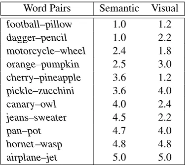
Initially, we created all possible pairings over McRae et al.’s (2005) nouns and computed their semantic relatedness using Patwardhan and Peder-sen (2006)’s WordNet-based measure. We opted for this specific measure as it achieves high corre-lation with human ratings and has a high coverage on our nouns. Next, for each word we randomly selected 30 pairs under the assumption that they are representative of the full variation of semantic similarity. This resulted in 7,576 word pairs for which we obtained similarity ratings using Ama-zon Mechanical Turk (AMT). Participants were asked to rate a pair on two dimensions, visual and semantic similarity using a Likert scale of 1 (highly dissimilar) to 5 (highly similar). Each task consisted of 32 pairs covering examples of weak to very strong semantic relatedness. Two con-trol pairs from Miller and Charles (1991) were in-cluded in each task to potentially help identify and eliminate data from participants who assigned ran-dom scores. Examples of the stimuli and mean ratings are shown in Table 2.
The elicitation study comprised overall 255 tasks, each task was completed by five volun-teers. The similarity data was post-processed so as to identify and remove outliers. We consid-ered an outlier to be any individual whose mean pairwise correlation fell outside two standard de-viations from the mean correlation. 11.5% of the annotations were detected as outliers and re-moved. After outlier removal, we further ex-amined how well the participants agreed in their similarity judgments. We measured inter-subject agreement as the average pairwise correlation co-efficient (Spearman’sρ) between the ratings of all annotators for each task. For semantic similarity, the mean correlation was 0.76 (Min=0.34, Max
5Available from http://homepages.inf.ed.ac.uk/
Word Pairs Semantic Visual
football–pillow 1.0 1.2
dagger–pencil 1.0 2.2
motorcycle–wheel 2.4 1.8
orange–pumpkin 2.5 3.0
cherry–pineapple 3.6 1.2
pickle–zucchini 3.6 4.0
canary–owl 4.0 2.4
jeans–sweater 4.5 2.2
pan–pot 4.7 4.0
hornet–wasp 4.8 4.8
[image:7.595.87.279.61.229.2]airplane–jet 5.0 5.0
Table 2: Mean semantic and visual similarity rat-ings for the McRae et al. (2005) nouns using a scale of 1 (highly dissimilar) to 5 (highly similar).
=0.97, StD=0.11) and for visual similarity 0.63 (Min=0.19, Max =0.90, SD =0.14). These re-sults indicate that the participants found the task relatively straightforward and produced similarity ratings with a reasonable level of consistency. For comparison, Patwardhan and Pedersen’s (2006) measure achieved a coefficient of 0.56 on the dataset for semantic similarity and 0.48 for vi-sual similarity. The correlation between the aver-age ratings of the AMT annotators and the Miller and Charles (1991) dataset wasρ=0.91. In our experiments (see Section 5), we correlate model-based cosine similarities with mean similarity rat-ings (again using Spearman’sρ).
Categorization The task of categorization (i.e., grouping objects into meaningful categories) is a classic problem in the field of cognitive science, central to perception, learning, and the use of language. We evaluated model output against a gold standard set of categories created by Fountain and Lapata (2010). The dataset contains a classification, produced by human participants, of McRae et al.’s (2005) nouns into (possibly multiple) semantic categories (40 in total).6
To obtain a clustering of nouns, we used Chi-nese Whispers (Biemann, 2006), a randomized graph-clustering algorithm. In the categorization setting, Chinese Whispers (CW) produces a hard clustering over a weighted graph whose nodes cor-6The dataset can be downloaded from http:
//homepages.inf.ed.ac.uk/s0897549/data/.
respond to words and edges to cosine similarity scores between vectors representing their mean-ing. CW is a non-parametric model, it induces the number of clusters (i.e., categories) from the data as well as which nouns belong to these clusters. In our experiments, we initialized Chinese Whis-pers with different graphs resulting from different vector-based representations of the McRae et al. (2005) nouns. We also transformed the dataset into hard categorizations by assigning each noun to its most typical category as extrapolated from human typicality ratings (for details see Foun-tain and Lapata, 2010). CW can optionally ap-ply a minimum weight threshold which we opti-mized using the categorization dataset from Ba-roni et al. (2010). The latter contains a classifica-tion of 82 McRae et al. (2005) nouns into 10 cate-gories. These nouns were excluded from the gold standard (Fountain and Lapata, 2010) in our final evaluation.
We evaluated the clusters produced by CW us-ing the F-score measure introduced in the Se-mEval 2007 task (Agirre and Soroa, 2007); it is the harmonic mean of precision and recall defined as the number of correct members of a cluster di-vided by the number of items in the cluster and the number of items in the gold-standard class, re-spectively.
4.4 Comparison with Other Models
Throughout our experiments we compare a bi-modal stacked autoencoder against unibi-modal au-toencoders based solely on textual and visual in-put (left- and right-hand sides in Figure 1, respec-tively). We also compare our model against two approaches that differ in their fusion mechanisms. The first one is based on kernelized canonical cor-relation (kCCA, Hardoon et al., 2004) with a lin-ear kernel which was the best performing model in Silberer et al. (2013). The second one emulates Bruni et al.’s (2014) fusion mechanism. Specifi-cally, we concatenate the textual and visual vec-tors and project them onto a lower dimensional la-tent space using SVD (Golub and Reinsch, 1970). All these models run on the same datasets/items and are given input identical to our model, namely attribute-based textual and visual representations.
repre-Semantic Visual
Models T V T+V T V T+V
McRae 0.71 0.49 0.68 0.58 0.52 0.62
Attributes 0.58 0.61 0.68 0.46 0.56 0.58
SAE 0.65 0.60 0.70 0.52 0.60 0.64
SVD — — 0.67 — — 0.57
kCCA — — 0.57 — — 0.55
Bruni — — 0.52 — — 0.46
[image:8.595.318.513.62.216.2]RNN-640 0.41 — — 0.34 — —
Table 3: Correlation of model predictions against similarity ratings for McRae et al. (2005) noun pairs (using Spearman’sρ).
sentations constructed from low-level image fea-tures. In their model, the textual modality is represented by the 30K-dimensional vectors ex-tracted from UKWaC and WaCkypedia.7 The
visual modality is represented by bag-of-visual-words histograms built on the basis of clustered SIFT features (Lowe, 2004). We rebuilt their model on the ESP image dataset (von Ahn and Dabbish, 2004) using Bruni et al.’s (2013) publicly available system.
Finally, we also compare to the word embed-dings obtained using Mikolov et al.’s (2011) re-current neural network based language model. These were pre-trained on Broadcast news data (400M words) using the word2vec tool.8 We
re-port results with the 640-dimensional embeddings as they performed best.
5 Results
Table 3 presents our results on the word simi-larity task. We report correlation coefficients of model predictions against similarity ratings. As an indicator to how well automatically extracted at-tributes can approach the performance of clean hu-man generated attributes, we also report results of a distributional model induced from McRae et al.’s (2005) norms (see the row labeled McRae in the table). Each noun is represented as a vector with dimensions corresponding to attributes elicited by participants of the norming study. Vector compo-nents are set to the (normalized) frequency with which participants generated the corresponding at-tribute. We show results for three models, using all attributes except those classified as visual (T), only
7We thank Elia Bruni for providing us with their data. 8Available fromhttp://www.rnnlm.org/.
# Pair # Pair
1 pliers–tongs 11 cello–violin
2 cathedral–church 12 cottage–house
3 cathedral–chapel 13 horse–pony
4 pistol–revolver 14 gun–rifle
5 chapel–church 15 cedar–oak
6 airplane–helicopter 16 bull–ox
7 dagger–sword 17 dress–gown
8 pistol–rifle 18 bolts–screws
9 cloak–robe 19 salmon–trout
[image:8.595.72.291.63.197.2]10 nylons–trousers 20 oven–stove
Table 4: Word pairs with highest semantic and vi-sual similarity according to SAE model. Pairs are ranked from highest to lowest similarity.
visual attributes (V), and all available attributes (V+T).9 As baselines, we also report the
perfor-mance of a model based solely on textual attributes (which we obtain from Strudel), visual attributes (obtained from our classifiers), and their concate-nation (see row Attributes in Table 3, and columns T, V, and T+V, respectively). The automatically obtained textual and visual attribute vectors serve as input to SVD, kCCA, and our stacked autoen-coder (SAE). The third row in the table presents three variants of our model trained on textual and visual attributes only (T and V, respectively) and on both modalities jointly (T+V).
Recall that participants were asked to provide ratings on two dimensions, namely semantic and visual similarity. We would expect the textual modality to be more dominant when modeling se-mantic similarity and conversely the perceptual modality to be stronger with respect to visual sim-ilarity. This is borne out in our unimodal SAEs. The textual SAE correlates better with seman-tic similarity judgments (ρ = 0.65) than its vi-sual equivalent (ρ= 0.60). And the visual SAE correlates better with visual similarity judgments (ρ= 0.60) compared to the textual SAE (ρ= 0.52). Interestingly, the bimodal SAE is better than the unimodal variants on both types of similarity judg-ments, semantic and visual. This suggests that both modalities contribute complementary infor-mation and that the SAE model is able to extract a shared representation which improves general-ization performance across tasks by learning them
9Classification of attributes into categories is provided by
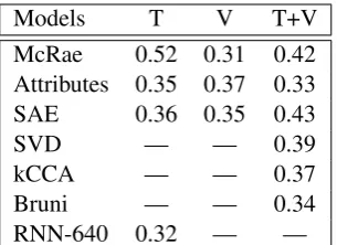
Models T V T+V
McRae 0.52 0.31 0.42
Attributes 0.35 0.37 0.33
SAE 0.36 0.35 0.43
SVD — — 0.39
kCCA — — 0.37
Bruni — — 0.34
[image:9.595.106.259.61.172.2]RNN-640 0.32 — —
Table 5: F-score results on concept categorization.
jointly. The bimodal autoencoder (SAE, T+V) outperforms all other bimodal models on both sim-ilarity tasks. It yields a correlation coefficient ofρ= 0.70 on semantic similarity andρ= 0.64 on visual similarity. Human agreement on the former task is 0.76 and 0.63 on the latter. Table 4 shows examples of word pairs with highest semantic and visual similarity according to the SAE model.
We also observe that simply concatenating textual and visual attributes (Attributes, T+V) performs competitively with SVD and better than kCCA. This indicates that the attribute-based representation is a powerful predictor on its own. Interestingly, both Bruni et al. (2013) and Mikolov et al. (2011) which do not make use of attributes are out-performed by all other attribute-based sys-tems (see columns T and T+V in Table 3).
Our results on the categorization task are given in Table 5. In this task, simple concatenation of vi-sual and textual attributes does not yield improved performance over the individual modalities (see row Attributes in Table 5). In contrast, all bimodal models (SVD, kCCA, and SAE) are better than their unimodal equivalents and RNN-640. The SAE outperforms both kCCA and SVD by a large margin delivering clustering performance similar to the McRae et al.’s (2005) norms. Table 6 shows examples of clusters produced by Chinese Whis-pers when using vector representations provided by the SAE model.
In sum, our experiments show that the bi-modal SAE model delivers superior performance across the board when compared against competi-tive baselines and related models. It is interesting to note that the unimodal SAEs are in most cases better than the raw textual or visual attributes. This indicates that higher level embeddings may be beneficial to NLP tasks in general, not only to those requiring multimodal information.
STICK-LIKE UTENSILS baton, ladle, peg, spatula,
spoon
RELIGIOUS BUILDINGS cathedral, chapel, church
WIND INSTRUMENTS clarinet, flute, saxophone,
trom-bone, trumpet, tuba
AXES axe, hatchet, machete,
toma-hawk
FURNITURE W/LEGS bed, bench, chair, couch, desk,
rocker, sofa, stool, table
FURNITURE W/O LEGS bookcase, bureau, cabinet,
closet, cupboard, dishwasher, dresser
LIGHTINGS candle, chandelier, lamp,
lantern
ENTRY POINTS door, elevator, gate
UNGULATES bison, buffalo, bull, calf, camel,
cow, donkey, elephant, goat, horse, lamb, ox, pig, pony, sheep
BIRDS crow, dove, eagle, falcon, hawk,
[image:9.595.306.529.62.299.2]ostrich, owl, penguin, pigeon, raven, stork, vulture, wood-pecker
Table 6: Examples of clusters produced by CW using the representations obtained from the SAE model.
6 Conclusions
In this paper, we presented a model that uses stacked autoencoders to learn grounded meaning representations by simultaneously combining tex-tual and visual modalities. The two modalities are encoded as vectors ofnatural language attributes
and are obtained automatically from decoupled
text and image data. To the best of our knowl-edge, our model is novel in its use of attribute-based input in a deep neural network. Experimen-tal results in two tasks, namely simulation of word similarity and word categorization, show that our model outperforms competitive baselines and re-lated models trained on the same attribute-based input. Our evaluation also reveals that the bimodal models are superior to their unimodal counterparts and that higher-level unimodal representations are better than the raw input. In the future, we would like to apply our model to other tasks, such as im-age and text retrieval (Hodosh et al., 2013; Socher et al., 2013b), zero-shot learning (Socher et al., 2013a), and word learning (Yu and Ballard, 2007).
References
Agirre, Eneko and Aitor Soroa. 2007. SemEval-2007 Task 02: Evaluating Word Sense Induc-tion and DiscriminaInduc-tion Systems. In Proceed-ings of the Fourth International Workshop on Semantic Evaluations. Prague, Czech Republic, pages 7–12.
Andrews, M., G. Vigliocco, and D. Vinson. 2009. Integrating Experiential and Distributional Data to Learn Semantic Representations. Psycholog-ical Review116(3):463–498.
Baroni, M., B. Murphy, E. Barbu, and M. Poe-sio. 2010. Strudel: A Corpus-Based Semantic Model Based on Properties and Types. Cogni-tive Science34(2):222–254.
Barsalou, Lawrence W. 2008. Grounded Cogni-tion.Annual Review of Psychology59:617–845. Bengio, Y., P. Lamblin, D. Popovici, and H. Larochelle. 2007. Greedy Layer-Wise Train-ing of Deep Networks. In Bernhard Sch¨olkopf, John Platt, and Thomas Hoffman, editors, Ad-vances in Neural Information Processing Sys-tems 19. MIT Press, pages 153–160.
Bengio, Yoshua. 2009. Learning Deep Architec-tures for AI. Foundations and Trends in Ma-chine Learning2(1):1–127.
Biemann, Chris. 2006. Chinese Whispers – an Ef-ficient Graph Clustering Algorithm and its Ap-plication to Natural Language Processing Prob-lems. In Proceedings of TextGraphs: the 1st Workshop on Graph Based Methods for Natu-ral Language Processing. New York, NY, pages 73–80.
Blei, D. M., A. Y. Ng, and M. I. Jordan. 2003. Latent Dirichlet Allocation.Journal of Machine Learning Research3:993–1022.
Bruni, E., G. Boleda, M. Baroni, and N. Tran. 2012a. Distributional Semantics in Technicolor. In Proceedings of the 50th Annual Meeting of the Association for Computational Linguistics. Jeju Island, Korea, pages 136–145.
Bruni, E., U. Bordignon, A. Liska, J. Uijlings, and I. Sergienya. 2013. Vsem: An open library for visual semantics representation. InProceedings of the 51st Annual Meeting of the Association for Computational Linguistics: System Demon-strations. Sofia, Bulgaria, pages 187–192.
Bruni, E., N. Tran, and M. Baroni. 2014. Multi-modal distributional semantics. J. Artif. Intell. Res. (JAIR)49:1–47.
Bruni, E., J. Uijlings, M. Baroni, and N. Sebe. 2012b. Distributional Semantics with Eyes: Us-ing Image Analysis to Improve Computational Representations of Word Meaning. In Proceed-ings of the 20th ACM International Conference on Multimedia. Nara, Japan, pages 1219–1228. Collobert, R., J. Weston, L. Bottou, M. Karlen, K. Kavukcuoglu, and P. Kuksa. 2011. Natural Language Processing (almost) from Scratch.
Journal of Machine Learning Research
12:2493–2537.
Deng, J., W. Dong, R. Socher, L. Li, K. Li, and L. Fei-Fei. 2009. ImageNet: A Large-Scale Hierarchical Image Database. In Proceedings of the IEEE Computer Society Conference on Computer Vision and Pattern Recognition. Mi-ami, Florida, pages 248–255.
Farhadi, A., I. Endres, D. Hoiem, and D. Forsyth. 2009. Describing Objects by their Attributes. In Proceedings of the IEEE Computer Soci-ety Conference on Computer Vision and Pat-tern Recognition. Miami Beach, Florida, pages 1778–1785.
Feng, Fangxiang, Ruifan Li, and Xiaojie Wang. 2013. Constructing Hierarchical Image-tags Bi-modal Representations for Word Tags Alter-native Choice. In Proceedings of the ICML 2013 Workshop on Challenges in Representa-tion Learning. Atlanta, Georgia.
Feng, Yansong and Mirella Lapata. 2010. Visual Information in Semantic Representation. In Hu-man Language Technologies: The 2010 Annual Conference of the North American Chapter of the Association for Computational Linguistics. Los Angeles, California, pages 91–99.
Finkelstein, L., E. Gabrilovich, Y. Matias, E. Rivlin, Z. Solan, G. Wolfman, and E. Ruppin. 2002. Placing Search in Context: The Concept Revisited. ACM Transactions on Information Systems20(1):116–131.
Golub, Gene and Christian Reinsch. 1970. Sin-gular Value Decomposition and Least Squares Solutions. Numerische Mathematik14(5):403– 420.
Griffiths, T. L., M. Steyvers, and J. B. Tenenbaum. 2007. Topics in Semantic Representation. Psy-chological Review114(2):211–244.
Hardoon, D. R., S. R. Szedmak, and J. R. Shawe-Taylor. 2004. Canonical Correlation Analy-sis: An Overview with Application to Learning Methods. Neural Computation 16(12):2639– 2664.
Harris, Zellig. 1970. Distributional Structure. In
Papers in Structural and Transformational Lin-guistics, pages 775–794.
Hinton, Geoffrey E. and Ruslan R. Salakhutdinov. 2006. Reducing the Dimensionality of Data with Neural Networks.Science313(5786):504– 507.
Hodosh, Micah, Peter Young, and Julia Hocken-maier. 2013. Framing Image Description as a Ranking Task: Data, Models and Evaluation Metrics. Journal of Artificial Intelligence Re-search47:853–899.
Huang, Jing and Brian Kingsbury. 2013. Audio-visual Deep Learning for Noise Robust Speech Recognition. In Proceedings of the 38th Inter-national Conference on Acoustics, Speech, and Signal Processing. Vancouver, Canada, pages 7596–7599.
Jones, R., B. Rey, O. Madani, and W. Greiner. 2006. Generating Query Substititions. In Pro-ceedings of the 15th International Conference on the World-Wide Web. Edinburgh, Scotland, pages 387–396.
Landau, B., L. Smith, and S. Jones. 1998. Object Perception and Object Naming in Early Devel-opment. Trends in Cognitive Science27:19–24. Landauer, Thomas and Susan T. Dumais. 1997. A Solution to Plato’s Problem: the Latent Seman-tic Analysis Theory of Acquisition, Induction, and Representation of Knowledge. Psychologi-cal Review104(2):211–240.
Lowe, D. 2004. Distinctive Image Features from Scale-invariant Keypoints. International Jour-nal of Computer Vision60(2):91–110.
Manning, C. D., P. Raghavan, and H. Sch¨utze. 2008. Introduction to Information Retrieval. Cambridge University Press, New York, NY.
McRae, K., G. S. Cree, M. S. Seidenberg, and C. McNorgan. 2005. Semantic Feature Pro-duction Norms for a Large Set of Living and Nonliving Things. Behavior Research Methods
37(4):547–559.
Mikolov, T., S. Kombrink, L. Burget, J. ˇCernock´y, and S. Khudanpur. 2011. Extensions of Recur-rent Neural Network Language Model. In Pro-ceedings of the 2011 IEEE International Con-ference on Acoustics, Speech, and Signal Pro-cessing. Prague, Czech Republic, pages 5528– 5531.
Mikolov, T., Wen-tau Yih, and G. Zweig. 2013. Linguistic Regularities in Continuous Space Word Representations. In Proceedings of the 2013 Conference of the North American Chap-ter of the Association for Computational Lin-guistics: Human Language Technologies. At-lanta, Georgia, pages 746–751.
Miller, George A. and Walter G. Charles. 1991. Contextual Correlates of Semantic Similarity.
Language and Cognitive Processes6(1). Nelson, D. L., C. L. McEvoy, and T. A.
Schreiber. 1998. The University of South Florida Word Association, Rhyme, and Word Fragment Norms.
Ngiam, Jiquan, Aditya Khosla, Mingyu Kim, Juhan Nam, Honglak Lee, and Andrew Ng. 2011. Multimodal Deep Learning. In Pro-ceedings of the 28th International Conference on Machine Learning. Bellevue, Washington, pages 689–696.
Patwardhan, Siddharth and Ted Pedersen. 2006. Using WordNet-based Context Vectors to Es-timate the Semantic Relatedness of Concepts. In Proceedings of the EACL 2006 Workshop on Making Sense of Sense: Bringing Compu-tational Linguistics and Psycholinguistics To-gether. Trento, Italy, pages 1–8.
Ranzato, Marc’Aurelio and Martin Szummer. 2008. Semi-supervised Learning of Com-pact Document Representations with Deep Net-works. InProceedings of the 25th International Conference on Machine Learning. Helsinki, Finland, pages 792–799.
Regier, Terry. 1996. The Human Semantic Poten-tial. MIT Press, Cambridge, Massachusetts. Roller, Stephen and Sabine Schulte im Walde.
Textual, Cognitive and Visual Modalities. In
Proceedings of the 2013 Conference on Empir-ical Methods in Natural Language Processing. Seattle, Washington, pages 1146–1157.
Sebastiani, Fabrizio. 2002. Machine Learning in Automated Text Categorization. ACM Comput-ing Surveys34:1–47.
Silberer, C., V. Ferrari, and M. Lapata. 2013. Mod-els of Semantic Representation with Visual At-tributes. In Proceedings of the 51st Annual Meeting of the Association for Computational Linguistics. Sofia, Bulgaria, pages 572–582. Silberer, Carina and Mirella Lapata. 2012.
Grounded Models of Semantic Representation. InProceedings of the 2012 Joint Conference on Empirical Methods in Natural Language Pro-cessing and Computational Natural Language Learning. Jeju Island, Korea, pages 1423–1433. Socher, R., M. Ganjoo, C. D. Manning, and A. Y. Ng. 2013a. Zero-shot learning through cross-modal transfer. InAdvances in Neural Informa-tion Processing Systems 26, pages 935–943. Socher, R., Quoc V. Le, C. D. Manning, and A. Y.
Ng. 2013b. Grounded Compositional Seman-tics for Finding and Describing Images with Sentences. In Proceedings of the NIPS Deep Learning Workshop.
Socher, R., J. Pennington, E. H. Huang, A. Y. Ng, and C. D. Manning. 2011. Semi-Supervised Re-cursive Autoencoders for Predicting Sentiment Distributions. InProceedings of the 2011 Con-ference on Empirical Methods in Natural Lan-guage Processing. Edinburgh, Scotland, pages 151–161.
Srivastava, Nitish and Ruslan Salakhutdinov. 2012. Multimodal Learning with Deep Boltz-mann Machines. In Advances in Neural In-formation Processing Systems 25, pages 2231– 2239.
Steyvers, Mark. 2010. Combining Feature Norms and Text Data with Topic Models.Acta Psycho-logica133(3):234–342.
Szumlanski, S. R., F. Gomez, and V. K. Sims. 2013. A New Set of Norms for Semantic Re-latedness Measures. InProceedings of the 51st Annual Meeting of the Association for Compu-tational Linguistics. Sofia, Bulgaria, pages 890– 895.
Turney, Peter D. and Patrick Pantel. 2010. From Frequency to Meaning: Vector Space Models of Semantics. Journal of Artificial Intelligence Research37(1):141–188.
Vincent, P., H. Larochelle, I. Lajoie, Y. Bengio, and P. Manzagol. 2010. Stacked Denoising Au-toencoders: Learning Useful Representations in a Deep Network with a Local Denoising Cri-terion. Journal of Machine Learning Research
11:3371–3408.
von Ahn, Luis and Laura Dabbish. 2004. Labeling Images with a Computer Game. InProceedings of the SIGCHI Conference on Human Factors in Computing Systems. Vienna, Austria, pages 319–326.
Wu, Pengcheng, Steven C. H. Hoi, Hao Xia, Peilin Zhao, Dayong Wang, and Chunyan Miao. 2013. Online Multimodal Deep Similarity Learning with Application to Image Retrieval. In Pro-ceedings of the 21st ACM International Con-ference on Multimedia. Barcelona, Spain, pages 153–162.
Yih, Wen-tau, Ming-Wei Chang, Christopher Meek, and Andrzej Pastusiak. 2013. Question Answering Using Enhanced Lexical Semantic Models. In Proceedings of the 51st Annual Meeting of the Association for Computational Linguistics. Sofia, Bulgaria, pages 1744–1753. Yu, C. and D. H. Ballard. 2007. A Unified Model