Bilateral Export Demand Function of India: An Empirical Analysis

ISSN Online: 2162-2086 ISSN Print: 2162-2078

DOI: 10.4236/tel.2018.811151 Aug. 15, 2018 2330 Theoretical Economics Letters

Bilateral Export Demand Function of India: An

Empirical Analysis

Aruna Kumar Dash, Subhendu Dutta, Rashmi Ranjan Paital

Department of Economics, IBS Hyderabad (A Constituent of ICFAI Foundation for Higher Education), Hyderabad, India

Abstract

In this paper, we examine the determinants of bilateral export demand func-tion of India during 1993:Q1-2015:Q1. The starting point of our study is 1993:Q1 by keeping into consideration that RBI implemented market deter-mined managed floating flexible exchange rate system during that period. We have employed Auto Regressive Distributed Lag (ARDL) model by using the macroeconomic variables such as real exports, foreign income, nominal ex-change rate (Rupee-Dollar) and relative price. We found there exists a long run equilibrium relationship between real exports, foreign income, exchange rate and relative price. In our empirical analysis, we found that in the long run and short run, real exports are influenced more by foreign income fol-lowed by relative price. Foreign income carries a positive sign and is statisti-cally significant, which implies that 1% increase in foreign income will in-crease real export by 1.63% in the long run. Likewise, relative price carries a negative sign and is statistically significant which implies 1% decrease in rela-tive prices that will increase real exports by 0.22% in the long run. The no-minal exchange rate carries a negative sign and is statistically significant (in both short run and long run), which suggests that depreciation of nominal exchange rate would not stimulate the volume of export during our study pe-riod. Hence, for policy point of view if any policy makers want to promote exports by depreciating, the rupee will not give fruitful results.

Keywords

Export Demand Function, ARDL, India

1. Introduction

International trade has played an important role in the development of both de-veloped and developing countries as countries are dependent on each other due How to cite this paper: Dash, A.K., Dutta,

S. and Paital, R.R. (2018) Bilateral Export Demand Function of India: An Empirical Analysis. Theoretical Economics Letters, 8, 2330-2344.

https://doi.org/10.4236/tel.2018.811151

Received: June 12, 2018 Accepted: August 12, 2018 Published: August 15, 2018

Copyright © 2018 by authors and Scientific Research Publishing Inc. This work is licensed under the Creative Commons Attribution International License (CC BY 4.0).

DOI: 10.4236/tel.2018.811151 2331 Theoretical Economics Letters to uneven distribution of scarce resources. The role of international trade in the development of a country is undoubtedly undeniable. Perhaps more firmly es-tablished than the relationship between exports and growth is that between fluctuations in exports and cyclical variations in economic activity. If shifts in demand were the major factor, then a study of the demand function for exports will provide a fuller understanding of the causes of economic fluctuations [1].

India’s exports to the whole world are showing an increasing trend during the period 1993:Q1 to 2008:Q2. India’s exports have increased from 5682.49 million USD in 1993:Q1 to 56433.8 million USD in 2008:Q2. India’s exports have in-creased by 10 times during this period. India’s exports to the whole world started falling since 2008:Q2 (Figure 1). While exports are falling temporarily in the af-termath of the Global Financial Crisis which started in the USA and gradually spread across the world, the value of exports has remained essentially flat since 2011. Raissi and Tulin (2015) [2] quoted that global factors have adversely af-fected India’s exports, as potentially did the appreciation of the real effective ex-change rate. It is believed that exports play an important role in the growth of the economy. As India’s exports to the whole world are not showing an increas-ing trend which forces us to see whether India’s exports to the USA are increasincreas-ing or not as the USA is the major trading partner of India for a couple of decades.

India’s exports to the USA fall from 6210.94 million USD in 2008:Q4 to 4199.36 million USD 2009:Q2. Though USA remained as a major export partner of India, exports had fallen during 2008:Q4 which was because of Global Finan-cial Crisis. The volume of exports falls after some lags might be because of con-sumer response lag and weak concon-sumer confidence index. Since 2009:Q2 India’s exports to the USA picked up and were showing an increasing trend (Figure 2).

It is believed that export growth should play an important role in economic growth in developing countries. Given the importance of export expansion of

DOI: 10.4236/tel.2018.811151 2332 Theoretical Economics Letters Figure 2. India’s exports to USA (millions of USA Dollars). Source: Authors’ calculations.

growth and balance of payments’ concerns, the worrisome fact is that the Per-centage share of the India’s exports to the USA to the whole World has declined from 22.52% in 1999 to 13.38% in 2015 (Figure 3). Hence, it is a serious concern for the Indian economy as USA is the major export partner of India.

The trade policy announced in 2014 by the government envisaged total ex-ports of $900 billion by 2020, however, it would only be possible if exex-ports grow by 40% per annum from now on [3].

Another reason for which the study of export demand function of a country becomes important is the fact that many of the developing countries are on the brinks of balance of payments problems. Keeping in view the importance of ex-ports in the economic growth of a country, an attempt is made in this paper to examine the determinants of bilateral export demand function of India in short run and long run. As US is the major trading partner of India, we examine In-dia-USA bilateral trade relationship in aggregate level. Rahman et al. [4] pointed out that if bilateral responses to exchange rates and other variables that deter-mine trade flows differ, then aggregate trade flows yield misleading results. In addition, if the response of the trade flows to the real exchange rate varies by country with the nature of the trade, disaggregation will give a clear picture.

Given this backdrop, the study has two fold objectives. First, is to find out the determinants of bilateral export demand function of India in short run and long run. Second, is to identify that among the macroeconomic variables which vari-able plays an important role in affecting exports. Finally, we hope that the con-clusion of this paper will be helpful for policy makers to formulate trade policies and it will also stimulate scholars to conduct further research, which would be beneficial to policy makers in the future.

The paper is organized as follows. Following an introduction in Section I, Sec-tion II reviews a few selected literatures in this area. SecSec-tion III discusses model specification. Section IV highlights the methodology used. Variables defined and data sources are presented in Section V. Section VI highlights the empirical re-sults followed by conclusions and policy implications in Section VII.

DOI: 10.4236/tel.2018.811151 2333 Theoretical Economics Letters Figure 3. Percentage share of the India’s exports to the USA to the whole World. Source: Authors’ calculations.

2. Review of Studies

Considering the importance of international trade to economic growth and de-velopment, especially in third world countries, a number of empirical studies onthe determinants of export demand functions have been carried out.

The contributions by Orcutt in 1950 [5] and Houthakker and Magee in 1969 [6] were noteworthy. The level of real income and price competitiveness are the main factors impacting exports. While analyzing the models of export demand, Houthakker and Magee [6] found that in countries which were imported and in the countries which were exported, the level of real income and price competi-tiveness impacted exports significantly. Hatton [1] and Wong et al. [7] also opined that prices play an important role in the determination of exports for developing countries. Wong et al. [7] found that there is a unique long-run rela-tionship between quantities of export, relative price, real foreign income and real exchange rate variability in Malaysia. Foresta, James J. and Turnerb, Paul [8] al-so confirmed the relationship between aggregate exports, world trade and the-real exchange rate in their study of USA.

The concept of elasticity of foreign demand plays an important role in inter-national trade research. A major part of the interinter-national trade research is done in this area in the last 20 years. Exports respond significantly to changes in rela-tive prices. This is evident from the studies by Goldstein and Khan [9]; Hossain et al. [10]; Raissi et al. [11]; Cocar [12] and Islam [13]. Goldstein and Khan [9] found that in six of the eight countries, they studied had relatively elastic de-mand and supply. Hossain et al. [10] used the Pesaran bounds tests and the Jo-hansenco-integration tests in his study in Indonesia and found that the country’s exports had highly elastic demand in the long run. Cocar [12] applied panel unit root and co-integration tests and showed that the real exchange rate elasticity of total export demand is inelastic, whereas the income elasticity is relatively elastic in USA. Narayan et al. [14] re-estimated the import and the export demand

22.52

13.38

0 5 10 15 20 25

1993 1994 1995 1996 1997 1998 1999 2000 2001 2002 2003 2004 2005 2006 2007 2008 2009 2010 201

1

DOI: 10.4236/tel.2018.811151 2334 Theoretical Economics Letters functions for Mauritius and South Africa using time series data and found that there is a long-run relationship between import demand, income and prices for both countries. Islam [13] found that GDP, exchange rate and inflation rateare important determinants for foreign trade of Bangladesh. Bolaji et al. [15] con-firmed a uni-causal link from export to growth in Nigeria.

Non-price factors such as patent applications and government and business characteristics of a country are also important factors for understanding of in-ternational competitiveness. Studies by Verheyen [16] revealed that these factors also have significant positive effects on export demand.

While most of the literature concentrates on developed economies, there is hardly few research carried out to examine the bilateral export demand function so far as emerging country like India is concerned. For instance, Raissi et al. [11] studied the short-term and long-run price and income elasticity of Indian ex-ports and found that international relative-price competitiveness, world de-mand, and energy shortages had considerable bearing on Indian exports. Ta-keshi I. [17] examines an empirical analysis of the aggregate export demand function in post-liberalization India. The empirical results indicate that all es-timated coefficients are statistically significant with expected signs and that the absolute value of the coefficient is the largest for the world price, followed by world income and domestic income. Further, the results reveal that price competitiveness has improved India’s export market. Moreover, the statisti-cally significant world income elasticity suggests that the global economic boom may contribute to an increase in India’s exports, whereas the global re-cession has likely had an adverse impact on the Indian economy through its trade channel.

We believe that these studies are not sufficient enough so far as emerging country like India is concerned. These studies are not sufficient enough to reach any definite conclusion. Hence, any new study will add to the review of litera-ture. By keeping this in our mind, the present study is carried out to investigate the bilateral export demand function of India by applying the ARDL model and using the latest data available. We believe, our study will throw some light to the policy makers and for the scope of future research.

3. Model Specification

Export demand of a country is affected by two important factors. These are—1) foreign income, which is an indicator of the economic activity and purchasing power of trading partner, and 2) terms of trade (or competitiveness effect), which depends on the ratio of the respective price levels and the nominal ex-change rate. The econometric model presented below for the empirical study shows a standard long-run relationship between real exports, nominal exchange rate, relative price and foreign income.

0 1 2 3

t t t t t

DOI: 10.4236/tel.2018.811151 2335 Theoretical Economics Letters where, Export (Ext) = real exports of India at time t; Foreign Income (Fyt) = foreign economic activity at time t; Exchange rate (Eratet) = nominal exchange rate at time t (Rupee per unit of USD); Relative price (Rpt) = relative price (which is a measure of competitiveness) at time t; ut = the normally distributed error term with all classical properties.

As exports depend on the foreign country’s income, we expect a positive sign for the coefficient of foreign country’s income. However, if rise in real income is due to an increase in the production of import substitute goods, imports may decline as income increases in which case the coefficient of income in foreign country would be negative. The increase in nominal exchange rate (i.e. deprecia-tion of the exchange rate) makes domestic goods cheaper in other countries, which increases the competitiveness of domestic goods in the international markets, raising their demand. So we expect the coefficient of the exchange rate to be positive. A fall in the relative price of a country will cause the domestic goods to be more competitive as compared to foreign goods, which would result in an increase in exports and decrease in imports and vice versa. Therefore, we expect the coefficient of relative price to be negative.

The above equation includes constant/intercept term “β_{0” because there will}

be some exports even if all other variables are zero. β1, β2, and β3 are the elastici-ty coefficients with respect to the variables FY ERATE RP_t, _t, _t respectively. Ut is the residual term, which shows the affects of other variables on exports not in-cluded in the model.

The exchange rate variable used here is the nominal exchange rate. We point out that the model uses nominal exchange rates, and not real exchange rate, though it is the real exchange rate that is normally understood to affect the volume of trade. We have divided real exchange rate into its two components of nominal exchange rate and relative price level. The reason for analyzing these components separately is that the volume of trade responses to real ex-change rate ex-changes may differ according to whether the real exex-change rate changes are due to nominal exchange rate changes or the changes in relative price level.

4. Research Methodology

Before proceeding for empirical estimation, each of the macroeconomic va-riables is initially tested for their stationarity properties and order of integration. The Augmented Dickey Fuller (ADF) and Phillips Perron (PP) test is used for this purpose. Subsequently, the bound testing approach to ARDL model devel-oped by Pesaran, Shin and Smith [18] is used to check if the variables are coin-tegrated or not. We apply ARDL bounds testing approach developed by Pesaran

et al. [18]. This approach has a number of advantages as compared to Johansen

DOI: 10.4236/tel.2018.811151 2336 Theoretical Economics Letters order. However, the ARDL approach does not require variable to be integrated of the same order. It can be applied whether the variables are purely I (0) or I (1) or mutually cointegrated. Thirdly, the ARDL approach provides unbiased long run estimates with valid t-statistics if some of the model regressors are endo-genous [21] [22]. Fourthly, this approach provides a method of assessing short run and long run effects of one variable on the other simultaneously and it is al-so separates short run and long run effects (Bentzen and Engsted, 2001) [23]. Another significant advantage of ARDL approach over the cointegration tech-nique is that different variables can be assigned different lag length in the ARDL model.

The following ARDL model is estimated to check for the presence of cointe-gration. ARDL model is used to investigate the relationship between the real ex-ports, foreign income, nominal exchange rate and relative price. The model spe-cification is as follows:

0 1 1 2 1 3 1 4 1

5 6 7

1 0 0

8 1 1

0

ln ln ln ln ln

ln ln ln

ln

t t t t t

n n n

i t i i t i i t i

i i i

n

i t i t t

i

Ex Ex Fy Erate Rp

Ex Fy Erate

Rp EC e

α α α α α

α α α

α π

− − − −

− − −

= = =

− −

=

∆ = + + + +

+ ∆ + ∆ + ∆

+ ∆ + +

∑

∑

∑

∑

(2)

The existence of a cointegrated relationship between the variables in the above mentioned ARDL model specifications is examined with the help of F or Wald test statistics. The Wald test examines the joint null hypothesis of zero cointe-gration between the variables, against the alternative hypothesis of the presence of cointegration. The calculated F-statistics are compared with two sets of criti-cal values computed by Pesaran, Shin and Smith [18] for a given level of signi-ficance in their bound testing approach to the analysis of the long-run relation-ship. If the computed Wald F statistics exceed/fall above the upper critical value, it implies that all the variables are cointegrated i.e. I (1), and the null hypothesis of zero cointegration can be rejected. On the other hand, if the computed Wald F statistics fall below the lower bounds critical value, it implies that all the va-riables are not cointegrated, i.e. I (0), and in this context the null hypothesis of zero cointegration can’t be rejected. However, if the calculated Wald F statistics fall between the lower and upper bound of critical values, the tests become in-conclusive. If the null hypothesis of zero cointegration is rejected then the ARDL model is estimated to study the short run dynamics. The error correction term measures the speed with which the deviation from the long run equilibrium is corrected in each period and error correction term is expected to have a negative sign and statistically significant.

DOI: 10.4236/tel.2018.811151 2337 Theoretical Economics Letters of heteroscedasticity of the unknown, general form. Jarque Bera (J-B) test is used to test the null hypothesis that the residuals are normally distributed. Parameter stability tests play a pivotal role to ensure reliability of policy simulations based on the model. To test for parameter stability, we have applied the CUSUM (Cumulative Sum) and Cumulative Sum of Squires (CUSUMQ) tests developed by Brown, Durbin and Evans in1975 [24]. CUSUM and CUSUMQ test are car-ried out to check for parameter stability in the estimated ARDL model. This test plots the cumulative sum together with the 5% critical lines. Movement outside the 5% critical lines indicates parameter instability. The test finds no evidence of major parameter instability since the cumulative sum test statistics do not cross the 5% critical lines. Stability of the estimated elasticities suggests that the model can be considered stable enough for forecasting and policy analysis.

5. Variables Defined and Data Sources

We used India’s monthly exports to the USA (in USD) divided by the unit value of export price in the respective month to generate data on monthly real ex-ports. The time series data of unit value of export price is not available on a monthly basis. Hence, we interpolated yearly unit value of export price into a monthly unit value of export price through quadratic method which is exten-sively used by many researchers. Though the volume of exports is expressed in USD million and rupee terms in Indian context, we prefer exports in USD mil-lion terms rather than the rupee term as USD fluctuates less compared to ru-pee. In addition to that, the USD is treated as one of the safe haven currencies in the international market. Unit values of exports indices are treated as price indices of exports. It is used as a deflator to compute the volume of exports from value of exports. Economic theory tells that foreign income is an impor-tant determinant of exports. We have used USAGDP to represent foreign in-come. The relative price (which is a measure of competitiveness) is measured by the ratio of India’s unit value of exports to USA CPI. Finally, the study uses the bilateral Rupee-Dollar nominal exchange rate as it is widely believed that exchange rate also plays an important role in affecting exports and imports of a country.

DOI: 10.4236/tel.2018.811151 2338 Theoretical Economics Letters

6. Empirical Results

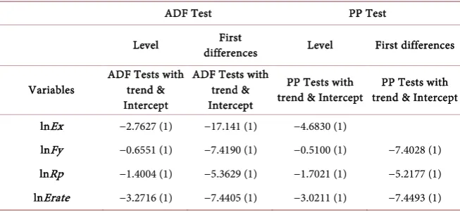
Table 1 presents the results of ADF and PP tests for examining the stationarity properties of macro-economic variables. The optimal lag length for carrying out the ADF and PP test for each of the variables is chosen on the basis of Akaike Information Criteria (AIC). It is observed from Table 1 that all the variables are non-stationary at level except exchange rate. Hence, we can say that variables are integrated of order 0, i.e. I (0). However, all the variables become stationary only at first differences that is, they are integrated of order 1 or I (1). Since, the ma-croeconomic variables are found to be I (1), the bound testing approach to ARDL model is implemented to check for the presence of any cointegrating rela-tionship among the variables. The ARDL approach to cointegration cannot be applied if any of the variables is found to be I (2).

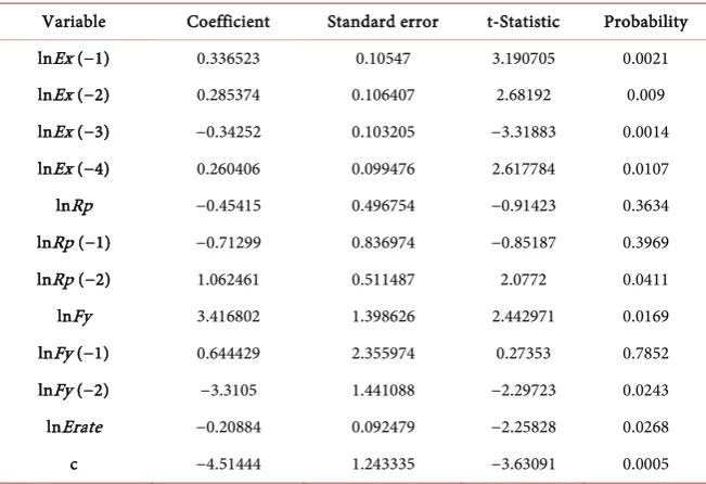
Table 2 shows the results of ARDL model which includes both lags and cur-rent variables. The ARDL (4, 2, 2, 0) model is chosen based on Akaike Infor-mation Criteria (AIC). In ARDL (4, 2, 2, 0) model for lag 4 corresponds to the variable LNEX, Lag 2, corresponds to LNRP, FY corresponds to Lag 2 and Lag 0 corresponds to LNERATE. After estimating ARDL model, then we proceed to check the cointegration test. The ARDL cointegration test is reported in Ta-ble 3.

The bound testing approach to cointegration is reported in Table 3. When Wald test is performed for ARDL model, the F-statistic is found to be 4.6528. Since the computed F-statistics exceeds the critical upper bound at 5% level sig-nificance, the null hypothesis of zero cointegration can be rejected. This implies there exists a long run equilibrium relationship between exports, foreign income, exchange rate and relative price.

The long run coefficient estimated from ARDL model is reported in Table 4.

Table 1. Unit root test.

ADF Test PP Test

Level _differences First Level First differences

Variables ADF Tests with trend & Intercept

ADF Tests with trend & Intercept

PP Tests with

trend & Intercept trend & Intercept PP Tests with

lnEx −2.7627 (1) −17.141 (1) −4.6830 (1)

lnFy −0.6551 (1) −7.4190 (1) −0.5100 (1) −7.4028 (1)

lnRp −1.4004 (1) −5.3629 (1) −1.7021 (1) −5.2177 (1)

lnErate −3.2716 (1) −7.4405 (1) −3.0211 (1) −7.4493 (1)

DOI: 10.4236/tel.2018.811151 2339 Theoretical Economics Letters Table 2. ARDL model.

Variable Coefficient Standard error t-Statistic Probability

lnEx (−1) 0.336523 0.10547 3.190705 0.0021

lnEx (−2) 0.285374 0.106407 2.68192 0.009

lnEx (−3) −0.34252 0.103205 −3.31883 0.0014

lnEx (−4) 0.260406 0.099476 2.617784 0.0107

lnRp −0.45415 0.496754 −0.91423 0.3634

lnRp (−1) −0.71299 0.836974 −0.85187 0.3969

lnRp (−2) 1.062461 0.511487 2.0772 0.0411

lnFy 3.416802 1.398626 2.442971 0.0169

lnFy (−1) 0.644429 2.355974 0.27353 0.7852

lnFy (−2) −3.3105 1.441088 −2.29723 0.0243

lnErate −0.20884 0.092479 −2.25828 0.0268

c −4.51444 1.243335 −3.63091 0.0005

Note: R Squared 0.9554, Adjusted R Squared 0.9492, Durbin Watson Test 1.82, Probability F statistic 0.0000. Source: Authors’ calculations.

Table 3. Results of ARDL Cointegration test (Bounds Testing to Cointegration).

Optimal Lag Lengeth (4, 2, 2, 0) F-Statistics (Wald Test) 4.6528

Critical Values (T = 89)

Lower bounds I (0) Upper bounds I (1)

1 Percent Level 4.29 5.61

5 Percent level 3.23 4.35*

10 percent level 2.72 3.77

Note: * denotes 5% level of significance. Source: Authors’ calculations.

Table 4. Estimated long run coefficient using the ARDL approach.

Regressor Coefficient Standard Error t-Statistics Probability

lnRp −0.22746 0.130538 −1.74246 0.0854

lnFy 1.631253 0.181066 9.009158 0.0000

lnErate −0.45379 0.231529 −1.95998 0.0536

C −9.80941 1.252608 −7.83119 0

Source: Authors’ calculations.

DOI: 10.4236/tel.2018.811151 2340 Theoretical Economics Letters 0.22%. Foreign income measures the economic activity and purchasing power of the trading partners. The expected signs of the coefficient of foreign income could be positive or negative. Economic theory suggests that the volume of ex-ports to a foreign country ought to increase as the real income and purchasing power of the foreign countries rises and vice-versa. An increase in foreign in-come will lead to foreigners’ importing more goods from the domestic countries and hence the coefficient of foreign income is positive. However, if increase in foreign income is associated with an increase in production of import substitute goods, domestic country’s exports will fall and in that case coefficient of foreign income carries the negative sign. In our empirical analysis we found that foreign income carries a positive sign and is statistically significant, which implies that 1% increase in foreign income will increase real export by 1.63%. The nominal ex-change rate carries a negative sign and is statistically significant which suggest that depreciation of nominal exchange rate would not stimulate the volume of export. On Table 4, we can conclude that in the long run, real exports are influenced more by foreign income followed by nominal exchange rate and relative price.

The short run dynamics of ARDL model is shown in Table 5. In the short run, the relative price is negatively related to real export which implies that a 1% decrease in relative prices will increase real exports by 1.06% at one lag. In the short run, current relative price has no import on real export. This might be be-cause of consumer response lag, production lag etc. The foreign income has a positive impact to real export. A 1% increase in foreign income increases real exports by 3.41% in the current period. When foreign country’s income increas-es, foreign people are better off and their standard of living enhanced which al-lows them to demand more imports. The nominal exchange coefficient carries the negative sign and statistically significant in the short run. This implies that depreciation of Indian rupee will promote exports during our study period. The error correction term is found to be negative and statistically significant, pro-viding further empirical evidence in support of the presence of cointegration between the variables. ECT value of −0.46 implies that about 46% of the short run disequilibrium between these variables is corrected every quarter.

Table 5. Short run representation of ARDL model.

Regressor Coefficient Standard Error t-statistics Probability

ΔlnEx (−1) −0.20326 0.12161 −1.67142 0.0987

ΔlnEx (−2) 0.082113 0.118019 0.695759 0.4887

ΔlnEx (−3) −0.26041 0.099476 −2.61778 0.0107

ΔlnRp −0.45415 0.496754 −0.91423 0.3634

ΔlnRp (−1) −1.06246 0.511487 −2.0772 0.0411

ΔlnFy 3.416802 1.398626 2.442971 0.0169

ΔlnFy (−1) 3.310503 1.441088 2.297226 0.0243

ΔlnErate −0.20884 0.092479 −2.25828 0.0268

ECMt−1 −0.46022 0.127534 −3.60856 0.0005

DOI: 10.4236/tel.2018.811151 2341 Theoretical Economics Letters Model Robustness check

We want to check whether our dependent variable that is export is stable or not. For robustness checkour results, we did CUSUM and CUSUM squire test, serial correlation and Heteroscedasticity Test which is shown in Figure 4 and Figure 5 and Table 6 and Table 7 respectively.

Figure 4 plots the results of CUSUM tests for ARDL (4, 2, 2, 0) model and Figure 5 plots the results of CUSUMQ tests for ARDL (4, 2, 2, 0) model. In both Figure 4 and Figure 5, if the blue line is located within the two red lines, it im-plies that our dependent variable (export) is a stable variable. On the contrary, if the blue line is located outside of the two red lines, it implies that our dependent variable (export) is not a stable variable and model can’t be used for policy im-plications and can’t be reliable. Both CUSUM and CUSUMQ test finds no evi-dence of major parameter instability since the cumulative sum test statistics do not cross the 5% critical lines. Both CUSUM and CUSUMQ tests are found to lie within the 5% critical lines, indicating parameter stability is present in our mod-el. Stability of the estimated elasticities suggests that the model can be consi-dered stable enough for forecasting and policy analysis.

Breusch-Godfrey test is used to check whether the presence/absence of serial correlation in the data. Table 6 presents the Breusch-Godfrey Serial Correlation LM Test. If the error term is serially correlated, the estimated OLS standard er-rors are invalid and estimated coefficients will be biased and inconsistent due to the presence of a lagged dependent variable on the right hand side. The null hy-pothesis of the test is that there is no serial correlation in the residual. In Table 6 we found that there is no serial correlation exists in our data.

Table 7 presents heteroscedasticity test. White test is used to test the null hy-pothesis that errors are homoskedastic and independent of the regressions, against the alternative hypothesis of presence of hetroskedasticity of the un-known, general form. In Table 7, White test shows that there is no heteroscedas-ticity present in our data.

Figure 4. Cumulative sum of recursive residuals. Note: The straight line represent critical bounds at 5% level of significance. Source: Authors’ calculations.

-30 -20 -10 0 10 20 30

1996 1998 2000 2002 2004 2006 2008 2010 2012 2014

DOI: 10.4236/tel.2018.811151 2342 Theoretical Economics Letters Figure 5. Cumulative sum of squires of recursive residuals. Note: The straight line represents critical bounds at the 5 % level of significance. Source: Authors’ calculations.

Table 6. Breusch-Godfrey serial correlation LM test.

F-statistic 8.021769 Prob. F (2, 75) 0.2137

Obs*R-squared 15.68343 Prob. Chi-Square (2) 0.1004

Source: Authors’ calculation.

Table 7. Heteroscedasticity test: white.

F-statistic 1.261096 Prob. F (58, 30) 0.2477

Obs*R-squared 63.11375 Prob. Chi-Square (58) 0.3005

Scaled explained SS 36.17843 Prob. Chi-Square (58) 0.9891

Source: Authors’ calculation.

7. Conclusions and Policy Implications

In this paper, we examine the determinants of bilateral export demand function of India during 1993:Q1-2015:Q1. The study uses the ARDL model by using the macroeconomic variables such as real exports, foreign income, nominal ex-change rate and relative price. In our empirical estimation, we found that there exists a long run equilibrium relationship between real exports, foreign income, exchange rate and relative price. In the short run and long run, real exports are influenced more by foreign income followed by relative price. Foreign income carries positive sign and finds to be statistically significant, which implies that 1% increase in foreign income will increase real export by 1.63% in the long run. Likewise, relative price carries a negative sign and is statistically significant, which implies 1% decrease in relative prices will increase real exports by 0.22% in the long run. The nominal exchange rate carries a negative sign and is statis-tically significant (in both short run and long run), which suggests that deprecia-tion of nominal exchange rate would not stimulate the volume of export during our study period. Hence, for policy point of view if any policy makers want to promote exports by depreciating, the rupee will not give desirable results.

Ra--0.2 0.0 0.2 0.4 0.6 0.8 1.0 1.2

1996 1998 2000 2002 2004 2006 2008 2010 2012 2014

DOI: 10.4236/tel.2018.811151 2343 Theoretical Economics Letters ther, policy makers should focus more on controlling inflation for which our products will be more competitive in the international market and it will be helpful to boost our exports. Though foreign country’s income plays an impor-tant role in affecting real exports, policy makers have no control on foreign in-come and it is influenced by external factors.

Notwithstanding the current results provided useful information for policy-makers, this should be treated with caution. The study considered only USA, as it is listed on the top of all major trading partners of India since many decades. This is one of the limitations of the study, which provides further scope for fu-ture research. Moreover, the fufu-ture research has the scope to examine the bila-teral analysis of export demand function with India’s top 10 major trading part-ners, which would further contribute to the existing literature.

Conflicts of Interest

The authors declare no conflicts of interest regarding the publication of this paper.

References

[1] Hatton (1990) The Demand for British Exports, 1870-1913. Economic History Re-view, 43, 576-594. https://doi.org/10.2307/2596736

[2] Raissi, M. and Tulin, V. (2018) Price and Income Elasticity of Indian Exports-The Role of Supply-Side Bottlenecks. IMF Working Paper, WP/15/161, 1-16.

https://www.imf.org/external/pubs/ft/wp/2015/wp15161.pdf

[3] The Mint (2018) India Needs to Fundamentally Alter Its Export Strategy.

https://www.livemint.com/Opinion/rHODuZ18xX55H1tqPTBz2O/India-needs-to-f undamentally-alter-its-export-strategy.html

[4] Rahman, et al. (1997) Dynamics of the Yen-Dollar Real Exchange Rate and the US-Japan Real Trade Balance. Applied Economics, 29, 661-664.

https://doi.org/10.1080/000368497326868

[5] Orcutt, G. (1950) Measurement of Price Elasticities in International Trade. The Re-view of Economics and Statistics, 32, 117-132. https://doi.org/10.2307/1927649 [6] Houthakker, H.S. and Magee, S.P. (1969) Income and Price Elasticities in World

Trade. Review of Economics and Statistics, 51, 111-125.

https://doi.org/10.2307/1926720

[7] Wong, K.N. and Tang, T.C. (2011) Exchange Rate Variability and the Export De-mand for Malaysia’s Semiconductors: An Empirical Study. Applied Economics, 43, 695-706. https://doi.org/10.1080/00036840802599917

[8] Foresta, J.J. and Turnerb, P. (2013) Alternative Estimators of Co-Integrating Para-meters in Models with Nonstationary Data: An Application to USA Export De-mand. Applied Economics, 45, 629-636.

https://doi.org/10.1080/00036846.2011.608647

[9] Goldstein, M. and Khan, M.S. (1985) Income and Price Effects in Foreign Trade. In: Jones, R.W. and Kenen, P.B., Eds., Handbook of International Economics, Vol. 2 Elsevier Science, Amsterdam.

DOI: 10.4236/tel.2018.811151 2344 Theoretical Economics Letters

[11] Raissi, M. and Tulin, V. (2018) Price and Income Elasticity of Indian Exports-The Role of Supply-Side Bottlenecks. The Quarterly Review of Economics and Finance, 68, 39-45. https://doi.org/10.1016/j.qref.2017.11.003

[12] Coçar, E.E. (2002) Price and Income Elasticities of Turkish Export Demand: A Pan-el Data Application. Central Bank Review, 2, 19-53.

[13] Islam, T. (2016) An Empirical Estimation of Export and Import Demand Functions Using Bilateral Trade Data: The Case of Bangladesh. Journal of Commerce & Man-agement Thought,7, 526-551. https://doi.org/10.5958/0976-478X.2016.00030.6 [14] Narayan, S. and Narayan, P.K. (2010) Estimating Import and Export Demand

Elas-ticities for Mauritius and South Africa. Australian Economic Papers, 49, 241-252.

https://doi.org/10.1111/j.1467-8454.2010.00399.x

[15] Bolaji, Adelowkan, Oluwaseyi, Alimi and Olorunfemi (2018) Time Series Analysis of Non-Oil Export Demand and Economic Performance in Nigeria. Iranian Eco-nomic Review, 22, 295-314.

[16] Verheyen, F. (2015) The Role of Non-Price Determinants for Export Demand. In-ternational Economic Policy, 12, 107-125.

https://doi.org/10.1007/s10368-014-0281-z

[17] Takeshi, I. (2014) An Empirical Analysis of the Aggregate Export Demand Function in Post-Liberalization India. Global Economy Journal, 14, 1-10.

[18] Pesaran, M.H., Shin, Y. and Smith, R.J. (2001) Bounds Testing Approaches to the Analysis of Level Relationships. Journal of Applied Econometrics, 16, 289-326.

https://doi.org/10.1002/jae.616

[19] Johansen, S. and Juselius, K. (1990) Maximum Likelihood Estimation and Inference on Cointegration with Applications to the Demand for Money. Oxford Bulletin of Economics and Statistics, 52, 169-210.

https://onlinelibrary.wiley.com/doi/pdf/10.1111/j.1468-0084.1990.mp52002003.x

[20] Ghatak, S. and Siddiki, J. (2001) The Use of ARDL Approach in Estimating Virtual Exchange Rate in India. Journal of Applied Statistics, 28, 573-583.

https://doi.org/10.1080/02664760120047906

[21] Narayan, P.K. (2005) The Saving and Investment Nexus for China: Evidence from Cointegration Tests. Applied Economics, 37, 1979-1990.

https://doi.org/10.1080/00036840500278103

[22] Odhiambo, N.M. (2008) Energy Consumption and Economic Growth Nexus in Tanzania: An ARDL Bounds Testing Approach. Energy Policy, 37, 617-622.

https://doi.org/10.1016/j.enpol.2008.09.077

[23] Bentzen, I. and Engsted, T. (2001) A Revival of the Autoregressive Distributed Lag Model in Estimating Energy Demand Relationship. Energy, 26, 45-55.

https://www.sciencedirect.com/science/article/pii/S0360544200000529