Spline in Compression Methods for Singularly Perturbed 1D Parabolic Equations with Singular Coefficients

Spline in Compression Methods for Singularly Perturbed

1D Parabolic Equations with Singular Coefficients

Ranjan K. Mohanty1*, Vijay Dahiya2, Noopur Khosla3

1_{Department of Mathematics, Faculty of Mathematical Sciences, University of Delhi, New Delhi, India} 2_{Department of Mathematics, Deenbandhu Chhotu Ram University of Science & Technology, Murthal, India}

3_{Department of Mathematics, Bharati Vidyapeeth’s College of Engineering,} Guru Gobind Singh Indraprastha University, New Delhi, India

Email: *_{[email protected]}

Received January 16, 2012; revised February 20, 2012; accepted March 11, 2012

ABSTRACT

In this article, we discuss three difference schemes; for the numerical solution of singularity perturbed 1-D parabolic equations with singular coefficients using spline in compression. The proposed methods are of accurate and applicable to problems in both cases singular and non-singular. Stability theory of a proposed method has been dis-cussed and numerical examples have been given in support of the theoretical results.



2 2 O k h



1

Keywords: Spline in Compressions; Parabolic Equations; Two-Level Implicit Schemes; Singular Perturbation; Singular Coefficients; RMS Errors

1. Introduction

Consider the following singularly perturbed one space dimensional parabolic equation

 

 

 

= , , 0< <1, >0

xx t x

u u a x u b x u + f x t x t

   (1)

where0 and a



r

some positive constant K, and

 

 

x K0,

,



0

b x K fo f x t are continuous

bounded functions defined in the semi-infinite region

 



x t, 0 x 1,t0



    .

The initial and boundary conditions associated with Equation (1) are given by

 

,0 0

 

, 0 1

u x a x  x (2)

 

0, 0

   

, 1, 1

 

, 0

u t b t u t b t t (3)

We assume that the functions, a0

 

x , b t0

 

and b t1

 

are sufficiently smooth and their required high-order de-rivatives exist in the solution space .

This class of problems arise in various fields of science and engineering, for instance, fluid mechanics, quantum mechanics, optical control, chemical-reactor theory, aero-dynamics, geophysics etc. There are a wide variety of asymptotic expansion methods available for solving the problems of the above type. But there can be difficulties in applying these asymptotic expansions in the inner and outer regions, which are not routine exercises but require skill, insight and experimentations. In many applications

Equation (1) represents boundary or interior layers and has been studied by many authors. Henrici [1] has de-scribed the discrete variable methods for ordinary differ-ential equations. Ahlberg et al. [2] and Greville [3] have

worked on the theory of splines functions and their ap-plications. An introduction to singular perturbations was given by Malley [4]. Abrahamsson et al. [5] have

dis-cussed the finite difference approximations for the sys-tem of singularly perturbed ordinary differential equa-tions. Further Prenter [6], Boor [7], and Hemker and Miller [8] have studied various splines and variational methods to solve differential equations. A uniformly ac-curate difference method for a singular perturbation problem has been analyzed by Berger et al. [9]. Further,

Kreiss and Kreiss [10] and Segal [11] have discussed stable numerical methods for singular perturbation prob-lems. Later, Jain and Aziz [12] have derived an efficient numerical method for the solution of convection-diffu- sion equation using adaptive spline function approxima-tion. Miller et al. [13] have used piecewise uniform meshes

for upwind and central difference operators for solving singularly perturbed problems. Kadalbajoo and Patidar [14] have studied the spline in compression methods for the solution of a class of singularly perturbed two point boundary value problems. Later, Mohanty et al. [15]

have extended the work discussed in [14] and solved singularly perturbed two point singular boundary value problems. In 2005, Khan and Aziz [16] have discussed

the tension spline method for the solution of second order singularly perturbed boundary value problems. Khan et al. [17] have made a survey on various parametric spline

function approximations. However, the methods discussed in [17] are only applicable to problems in rectangular coordinates. In the past difficulties were experienced for the numerical solution of singularly perturbed one space dimensional parabolic problems in polar coordinates. The solution usually deteriorates in the vicinity of singularity. In recent past, Mohanty et al. [18] have derived new

sta-ble spline in tension methods for singularly perturbed one space dimensional parabolic equations with singular coefficients. In this paper, we have presented a new ap-proach based on spline in compression to solve singu-larly perturbed parabolic equations of type (1). We have refined our procedure in such a way that the solution retains its order and accuracy even in the vicinity of the singularity x = 0. It is well known that the most classical

methods fail when  is small relative to the mesh length

h > 0, that is used for discretization of the differential

Equation (1) in the x-direction. Our aim is to show that

compression splines can furnish accurate numerical ap-proximations of Equation (1), when all or any of the co-efficients a x

 

, b x





and f x t

 

, contain singularity at

x = 0 and when  is either small or large as compared

with h. We consider three types of problems. In the first

case, we analyze the problems in which the second de-rivative term uxx



x,t



and the function term u x t

 

, are

present, whereas the term containing the first term deriva-tive x is absent. The problems having the second

derivative

 

, term and first derivative term

t



,

xx

u x u x



t u_x

 

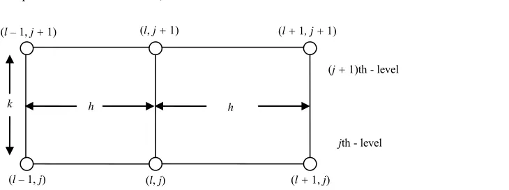
x,t

but lacking the function term are considered in the second case. Finally, the third case deals with the most general problems. In all cases, we use the continuity of first derivative of the spline function. The resulting spline difference methods are two-level implicit schemes (see Figure 1) and of accurate and are tri- diagonal system of equations at each advanced time level, which can be solved by using a tri-diagonal solver. The main significance of our work is that the proposed com-pression spline difference schemes are applicable to both singular and non-singular problems. In Section 2, we



u x



2 2 O k h



,t



have discussed the derivation of the spline methods and their application to singular problems. In Section 3, we have discussed stability analysis of a method. In Section 4, numerical results of three different singular problems have been given to demonstrate the utility of the proposed method. The numerical results confirmed that the pro-posed compression spline methods produce an oscilla-tion-free solution for 01 everywhere in the solu-tion region 0 < x < 1, t > 0.

2. Description of the Compression Spline

Method

The solution domain

  

0,1 t 0



is divided into



N 1



J mesh with the spatial step size h1



N1



in x-direction and the time step size k > 0 in t-direction

respectively, where N and J are positive integers. The

mesh ratio parameter is given by



2



₀

k h

 



.

Grid points are defined by



x tl, j







lh j,

J

k , l = 0(1) N + 1 and j0,1, 2, , . The notations u_lj and U_lj

are used for the discrete approximation and the exact solution of u x t

 

, at the grid point



x t_l, _j



,

respec-tively.

Let al a x

 

l ,bl b x

 

l and fl  f x

 

l

For x



xl₁,xl



, we denote



1





1



1



1 ˆ 1 ˆ

ˆ , ,

2 2

l l l l l l l l l l

a  a_ a b  b_ b f b_ b f₁fl



.

We consider the following three cases:

Case 1: First we consider the differential equation

 



 

, ,

0 1, 0, 0

xx t

u u b x u f x t x t b x

   

   



, (4)

which is a particular case of Equation (1) in which the first derivative term u_x

 

x t,

For the derivation of the method for the Equation (4), we follow the approaches given by Kadalbajoo and Pati-dar [14], and Mohanty et al. [15].

is absent.

Now we consider the ordinary differential equation

 

 

2

2

d _{, 0 1}

d

u

b x u f x x x

     (5)

h h

k

(l, j) (l + 1, j)

(l, j + 1)

(l – 1, j)

(l – 1, j + 1) (l + 1, j + 1)

[image:2.595.154.519.586.722.2]

jth - level (j + 1)th - level

The numerical solution of this equation is sought in the fo

Now using the approximations (12a)-(12c) in Equation (11) and neglecting high order terms we

pression spline scheme for the Equation fo

rm of the spline function S x

 

, which on each

inter-val



xl₁,xl



, denoted by Sl

 

x satisfies the

differen-tial equation

 

ˆ

 

ˆ

l l l

S x b S x f

    l (6)

The interpolating conditions:

,

 (7) and the continuity condition:

 ₍₈₎

Solving the Equation (6) and using co

 

1 1,

l l l

S x_ u_ S_l

 

x_l u_l

 

S_l x_l S_l

 

x_l .

the interpolating nditions (7), we get

 

_{ }

















1

1

S x Asin

sin

ˆ

sin

ˆ

l l l l

l

l

l l l

l

p x x hp

f B p x x

b  





  _

(9)

if

 _





l 1, l



x x_ x

where 1

ˆ ˆ ˆ

, ,

ˆl ˆl

l l l l l

l l

l

f f b

A u B u p

b  b 

    

Equation (9) is known as spline in compression, Re-placing l by l + 1 in Equation (9), we can obtain the

spline function Sl₁

 

x defined in



x xl, l1



.

 

_

_

















1 1 1

1

1

1 1 1

1

1 sin

ˆ

sin _ˆ

l l l l

l

l

l l l

l

A x

hp sin

S x p x

f B p x x

b

  





  





 _ 



  _

(10)

Differentiating Equation (9) with respect to “x” and

using the continuity condition (8), we obtain the spline in compression scheme for the numerical solution of Equa-tion (5) as:

















2

1 h 2

 _{ } 2

1 1 1 1

2 2

1 1 1 1

2

8 8

1 2 ,

8 4

1, 2, , .

l l l l l l l

l l l l l l

h

b b u b b b u

h h

b b u f f f

l N

 

 

   

   

 _{  } _{ } 

   

   

 

 _  _   

 

 

(11)

Note that, the scheme (11) is of O(h2) accurate for the

nu

(12a) merical solution of (5), however, the scheme fails to compute at l = 1. We overcome this difficulty by using

the following approximations:

1

l l

a_ a ha_xlO h

 

2 ,

 

2

1 ,

l l xl

b_  b hb O h (12b)

 

2

1 .

l l xl

f  f hf O h (12c)

obtain the (5) in compact rm:





2 2

1

1 2 2

8 l xl l 2 l l

h h

b hb u b u

  

   

    

   

   





 

2 2

1

1 2 ,

8

1 1

l xl l l

h h

b hb u f

l N

  

 

 _  _ 

 



(13)

In order to obtain the compression spline sch the parabolic Equation (4), we replace by

eme for

l

u 1



1



,

2

j j

l l

u  u

1

l

u_ by 1



j₁1 j₁



l l

u_ u_ , and f_l by

2





j j

tl l

u  f [where



,



2

j k

l l j

f  f x t  , and j



j1



obtain

j

tl  ul k] in (13) and

we

l

u u

















2 2 2

1 1

1 2

1 1

2 2 2

1

2 2

1

1

2 1

4 1

2

2 16

1 _{2 1}

2 16 4

1 _{2 .}

2 16

2 16

j j

l xl l l l

j

l xl l

j j

l xl l l l

j j

l xl l l

h h

b h u b

k h

b hb u

h h h

b hb u b u

k

h h

b hb u f

  



  

 

h

b  u 

 





  

     

   

  

 

_   _

 



   

 _   _   _  _

   

 

_   _ 

 

 

l1 1 N, j0,1, 2, (14)

Case 2: In this case, we consider the differential equa-tion of the form

 



 

, ,

   



This is a particular case of Equation (1), in which the function term

0 1, 0, 0.

xx t x

u u a x u f x t

x t a x

    (15)

 

,

u x t

vation

is absent.

For the deri of the method, we follow the same id

].

eas given by Kadalbajoo and Patidar [14], and Mo-hanty et al. [15

We consider the ordinary differential equation

 

f x

 

, 0 x 1, a x

 

0,

2

2

d u du

a x



d

dx  x    (16)

which is a steady-state case of Equation (15). As in case 1, we seek S(x) as a solution of the above diffe

equation

rential

 

_ˆ

 

ˆ

l l l l

S x a S x f

     (17) This satisfies the interpolating conditions (7) and the continuity condition (8).

we obtain

 









1

1

l l l l

L x L x

l l l

S x u e u e

F 1 1 1 ˆ 1 ˆ ˆ ˆ 1 , ˆ ˆ

l l l l

l

l

L x L x l

l l

l l

L x

l l

l l

l l l

f x e x e

F a

1

f f

u u h e x

F a a

           _   _    (18) where      



l 1, l



x x_ x , ˆl, l

a L



 and L xl l1 Ll l

l

F e  e x _.

Similarly, replacing l by l + 1 in Equation (18), we can

spline function in

get the Sl1

 

x valid



x xl, l1



.

 









1 1 1

1 1

1

1 L_l x_l L_l x_l

l l l

l

S x u e u e F          

1 1 1

1 1 1 1 1 1 1 1

1 1 1

ˆ 1 ˆ ˆ ˆ 1 . ˆ ˆ

l l l l

l

L x L x l

l l

l l

L x

l l

l l

l l l

f x e x e

F a

f f

u u h e x

F a a

                      _   _    (19)

Differentiating Equation (18) with respect to “x” and

using the continuity condition (8), we may obtain the spline in compression method for the approximate solu-tion of Equasolu-tion (16) as:





1 1

1 1 1

2 2 2

l l l

1 1 2 1 1 1 2 2 , 4 l l l l

l l l

p u

h

f f f

            _{ }      (20)

where . Note that, the scheme (20) is of O(h2)

accurate erical solution of (16), however, the scheme (20) fails to compute at l = 1. We overcome this

ty by us

p p p

u_   u

 _  _  _  _{ } 

 

     

  

l l

p hL

for the num

difficul ing the approximations defined by (12) and we obtain









 

2

1

1 2 ,

4

1 1 .

l xl l l

h h

a ha u f

l N         _  _     (21)

In order to obtain the compression spline meth the parabolic Equation (15), we replace by

2

1

1 2 2

4 l xl l 2 xl l

h h

a ha u a u

      _{ }  _{ }       od for l u



1



1 _,

2

j j

l l

u u ul1 by

 _



1



1 1 ,

2 ul ul and l

1 j j

f by



j j



tl l

u  f

[where j



,



l l j

k

f  f x t  , and

2





1

j j j

tl l

u  u_l u

















2 2 1 1 1 2 8 1 1 1 2 2 1 2 1 2 1 4 1 2 2 8 1 2 1

2 8 4

1

2 .

2 8

j j

l xl xl l

j

l xl l

l

j j

l xl l xl l

j j

l xl l l

h h h

a ha u a u

k h

a ha u

h h h

a ha u a u

k

h h

a ha u f

              _   _{ }   _   _        _   _  _  _       _   _   

 

l1 1 N j, 0,1, 2, (22)

Case 3: Finally we consider the most general problem (1), where both

         _   

 

, x u x t

ation of th

and are present. For the deriv e m we now follow the te

5].

 

,

u x t

ethod,

chniques given by Kadalbajoo and Patidar [14], and Mohanty et al. [1

For this purpose, we consider the ordinary differential equation

 

 

 

2 d d , d u u

a x b x u f x x

 2   

 

 

d

0 1, 0, 0

x

x a x b x

   

(23)

which is a steady-state case of (1). In this ca function

se the spline

 

S x satisfies

 

_ˆ

 

ˆ

 

ˆ

l l l l l l

S x a S x b S x f

      (24) This also satisfies the conditions (7) and (8). Solving the Equation (24) with the help of interpo

tions (7), we obtain

lating

condi- 

 





















ˆ l l c x S x e  1 1 ˆ sin ˆ ˆ sin sin ˆ

_ˆ , ,

l

l l l l l l

l

l l

l

h hd

G h d x x H h d x x

f

x x x

b      _    _   (25) where 1 ˆ ˆ 1 2 ˆ ˆ , , ˆ ˆ

ˆ _ˆ 1 _ˆ

ˆ , ˆ 4 ,

2 2

l l l l

c x c x

l l

l l l l

l l

l

l l l l

f f

G u e H u e

b b

a

c d a b

        _  _ _  _       

Replacing l by l + 1 in Equation (25), we can obtain

the spline function

k] in

(21) and we o taib n

 

1 l

S x for the Equation (24) in the

 

 





















1 1 ˆ l l c x S x e 1

1 1 1 1 1

1 1 1 ˆ sin ˆ ˆ sin sin ˆ

_ˆ ,

l

l l l l l l

l

l l

l

h hd

G h d x x H h d x x

f

x x x b            _    _   (26) Using the continuity condition (8), from Equation (25) we obtain the difference scheme based on spline in com-pression for the approximate solution of Equation (23



 





and (28) are of



2 2



O k h accurate for the numerical

solution of singularly perturbed parabolic partial differ-ential Equations (4), (15) and (1), respectively and free from the terms



1xl1



, hence very easily computed for

 

1 1 ,

l N j0,1, 2,, in the solution region .

3. Stability Analysis

Now we discuss the stability analysis for the scheme (14).

In this case the exact solution j l

U satisfies

) as 0 1 1 2 1 1 ( ) ,

l l l

l l l

r u r u r u h

q f q q f q f

  2   where          

 _    _ (27)

















2 2 1 1 1 1

0 2 2

1 1

1

2

1 , 2

4 2 4

2

1 , 2

4 2 4

1 2 , 4 2 1 . 2 l l

l l xl

l

l l

l l

l

l l l l

l

l

t p h

r p a

p

t p h

r p

p

r p p t t q

p q p                   _{  }               _                  , 1 , xl ha a ha

Note that the compression spline scheme (27) is of for the approximate solution of the Equation However, this scheme fails when the coefficients





















2 2 1 1 1 2 1 1 2 2 1 2 2

2 2 4

1

1 _{2 1}

2 16 4

1

2 2 16

1

2 1

2 16 4

1 ₂

2 16

j j

l xl l l l

j

l xl l

2

2

j j

l xl l l l

j j

l xl l l

h h

b hb U b U

k h

b hb U

h h

b hb U b U

k

h h

b hb U f O k h h

       h h                           _   _       _   _   _       _   _            (29)

we assume that there exists an error j j l  l u

j l

e U at

each grid point (xl, tj), then subtracting (14) from (29),

we obtain the error equation





















2 2 1 1 1 2 1 1 2 2 1 2

2 2 4

1

1

2 1

2 16 4

1 ₂

2 16 1

2 1

2 16 4

1 2 2 16 2 2 j j

l xl l l l

j

l xl l

j j

l xl l l

j

l xl l

h h

b hb e b e

k h

b hb e

h h

b hb e b e

k h

b hb e O k h h

      l h h                           _   _           _   _   _  _       _   _     (30)

 

2 O h

(23).

 

a x , b x

 

and f x

 

contain singularities and the

is to be determined at l = 1. We overcome this

difficulty by modifying the scheme (27) in such a manner he ion reta s order and accuracy even in the vicinity of the singularity x = 0.

As discussed in case 1 and case 2, using the approxi-mations (12) and neglecting high order terms, we obtain the following compression spline

solution

that t solut ins it

scheme for the solution of

To establish stability for the scheme (14), it is neces-sary to assume that the solution of the homogeneous part of the error Equation (30) is of the form j j i l,

l

e  e

where  is in general complex, i 1,  is real and we obtain the amplification factor

parabolic Equation (1) in compact form: see (28). Note that the compression spline schemes (14), (22)

















2 2 1 4

























2 2

1 2 1

1 2

2

2 1

1 2

2 2 2

2 2 1 2 2 1 4 16 1 4

2 4 32

1 _{4 1 4}

2 4 32 16

j 2

2 4 32

j

l l xl l l

j l

l xl l l

l

l xl l

j j

l

l xl l l l xl l l

h h

u a a b u

k ha h

a a b u

ha h h h

a a b u a a b u

k



ha h

a  a b 

                     _    _     _     _        _     _  _    _              









 

2 2 2 1 2

1 _{4 + , 1 1 , 0,1, 2, .}

2 4 32

j j

l

l xl l l l

ha h h

a  a b u f l N j

   

 

_     _  

  

2 2 2 3 2

2 2 2 3

2

2 1 sin ₂ sin

2 4 8

2 1 sin sin

2

2 4 8

l l xl

l l xl

h b h h b h b

i k

h b h h b h b

i k

 _

   



 _

   

   _{ } 

    

     

 

   

 



   _{ } 

   

    _{ } 

   

 

(31) For stability it is required that  1. Since

2

0 sin 1

2



 

 _{ }

  and  h, it is easy to verify from

(31) that  1for all variable angle  . Hence the heme (14) is unconditionally stable.

4. Experimental Results

Numerical results presented in this section are concerned with the application of the proposed spline in compres-sion methods to singular perturbation parabolic equat

We ngular bed

gu gion 0 , t > 0 for

a fixed value sc

ions. sin-have solved the following si ly pertur lar parabolic equations in the re < x < 1

of  k₂ 1.6. The right-hand-side

h 

s fu a

a test proce-

dure. In all cases, we have used Gauss-elimination me- thod (see Saad [19], Hageman and Young [20]) and a tri- diagonal solver to solve the problems. All computations were carried out using double length arithmetic.

Example 1:

homogeneou nctions, initial and bound ry conditions may be obtained using the exact solutions as

 

1 _{, , 0 1, 0}

xx t

u u u f x t x t

x

       (32)

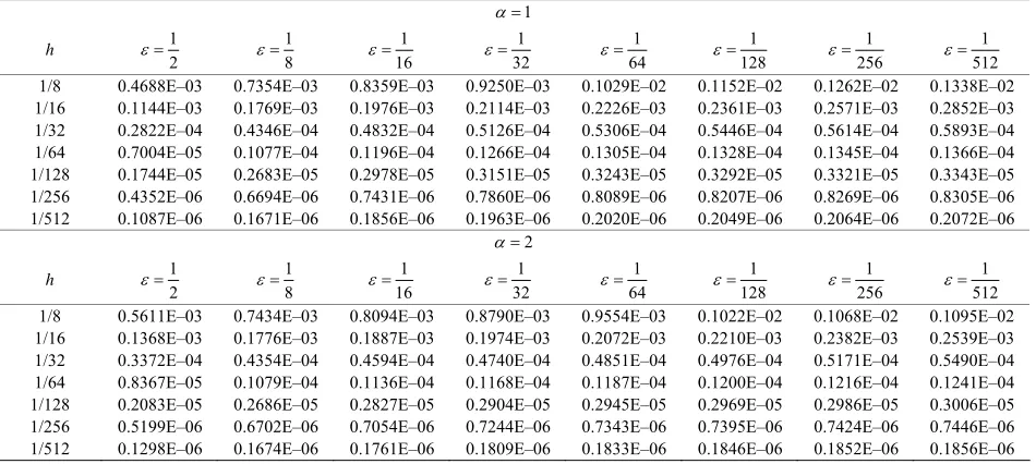
The exact solution is given by The root mean square (RMS) errors at lated in Table 1 for various values of

Example 2:

 

, tsin

u x t e hx.

t = 0.5 are

tabu-

0 1



  .

 

, , 0 1, 0

xx t x

u u u f x t x t

x 

       (33)

The exact solution is given by

 

, tcos h

u x t e x.

For  1 and perturbed

2, the equation above represents singu-bolic equation in

[image:6.595.67.535.401.497.2]

cy-pectively. Th Table 2 for different larly linear singular para

d spherical symmetry, res = 1.0 are tabulated in va

lindrical an errors at t

e RMS lues of 



01



and for  1 a

Example 3:

nd 2, respectively.



2



 

1

xx t x

u u u

x 1 x u f x t, , 0 x 1, t 0

         ₍₃₄₎

Table 1. The root mean square errors for example 1.

h 1

2

 1

8

 1

16

 1

32

 1

64

 1

128 

1/8 0.1167E–02 0.1716E–02 0.1808E–02 0.1863E–02 0.1902E–02 0.1930E–02

1/16 0.2924E–03 0.4454E–03 0.47

1/32 0.7286E–04 0.1129E–03 0.12

77E 39E

0.1814E–04 6E 3984E–04 E–04

1/128 0.4524E–05 0.7091E–05 0.7987E–05 –04 0.4743E–04 0.9120E–04

2E–05 0.2844E–05 0.1821E–04 0.5283E–04 –03 0.5054E–03 0.5344E–03 0.5615E–03 –03 0.1410E–03 0.1869E–03 0.3134E–03

–04 0. 0.9429 0.1684E–03

1/64 0.2835E–04 0.316

0.1088E

[image:6.595.62.537.525.738.2]

1/256 0.1129E–05 0.1771E–05 0.200

Table 2. The root mean square errors for example 2. 1



1 2

 1

8

 1

16

 1

32

 1

64

 1

128

 1

256

 1

51

h

2 

1/8 0.4688E–03 0.7354E–03 0.8359E–03 0.9250E–03 0.1029E–02 0.1152E–02 0.1262E–02 0.1338E–02

1/16 0.1144E 9E–03 03 0.222 – E–03

1/32 0.2822E 6E–04 04 0.530 – E–04

1/64 0.7004E 7E–04 04 0.130 – E–04

1/128 0.1744E 3E–05 05 0.324 – E–05

1/256 0.4352E 4E–06 06 0.808 – E–06

1/512 0.1087E 1E–06 06 0.202 – E–06

–03 0.176 0.1976E– 0.2114E–03 6E–03 0.2361E 03 0.2571 0.2852E–03

–04 0.434 0.4832E– 0.5126E–04 6E–04 0.5446E 04 0.5614 0.5893E–04

–05 0.107 0.1196E– 0.1266E–04 5E–04 0.1328E 04 0.1345 0.1366E–04

–05 0.268 0.2978E– 0.3151E–05 3E–05 0.3292E 05 0.3321 0.3343E–05

–06 0.669 0.7431E– 0.7860E–06 9E–06 0.8207E 06 0.8269 0.8305E–06

–06 0.167 0.1856E– 0.1963E–06

2 

0E–06 0.2049E 06 0.2064 0.2072E–06



1 2

 1

8 

h 1

16

 1

32

 1

64

 1

128

 1

256

 1

512 

1/8 0.5611E–03 0.7434E–03 0.8094E–03 0.8790E–03 0.9554E–03 0.1022E–02 0.1068E–02 0.1095E–02

1/16 0.1368E– 0.1776E–03 0.1887E– 3 0.1974E– 3 0.2072E– 3 0.2210E–03 0.2382E–03 0.2539E–03

1/32 0.3372E 0.4354E 4594E– 0.4740E– 0.4851E– 0.4976E– 5171E– 0.5490E–

03 –04

0 04

0 04

0 04

–04 0. 04 0. 04 04

1/64 0.8367E–05 0.1079E–04 0.1136E–04 0.1168E–04 0.1187E–04 0.1200E–04 0.1216E–04 0.1241E–04

1/128 0.2083E–05 0.2686E–05 0.2827E–05 0.2904E–05 0.2945E–05 0.2969E–05 0.2986E–05 0.3006E–05

1/256 1/512

0.5199E–06 0.1298E–06

0.6702E–06 0.1674E–06

0.7054E–06 0.1761E–06

0.7244E–06 0.1809E–06

0.7343E–06 0.1833E–06

0.7395E–06 0.1846E–06

0.7424E–06 0.1852E–06

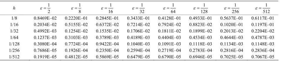
Table 3. The root mean square rors for exaer mple 3.

h 1

2

1 

8

1 

16

1 

32

1 

64

1 

128

1 

256

1 

512

1/8 0.8469E–02 0.2220E–01 0.2845E–01 0.3433E 1–0 0.4128E–01 0.4933E–01 0.5637E–01 0.6117E–01

1/16 0.2034E 02 0.5155E 02 0.6372E–02 0.7214E–02 0.7924E– 2 0.8823E– 1020E– 0.1197E– 1

1/32 0.4992E 03 0.1254E 02 0.1535E 2 0.1706E 2 0.1811E 2 0.1899E– 0.2013E– 0.2204E–

– –

– –

0 –0

02 0. 02

01 02

0 02

–0 –0

1/64 0.1237E–03 0.3103E–03 0.3789E–03 0.4189E–03 0.4404E–03 0.4534E–03 0.4644E–03 0.4787E–03

1/128 0.3080E–04 0.7724E–04 0.9422E–04 0.1040E–03 0.1091E–03 0.1118E–03 0.1134E–03 0.1148E–03

1/256 0.7686E–05 0.1926E–04 0.2350E–04 0.2594E–04 0.2719E–04 0.2783E–04 0.2816E–04 0.2836E–04

1/512 0.1919E–05 0.4812E–05 0.5869E–05 0.6479E–05 0.6790E–05 0.6946E–05 0.7025E–05 0.7067E–05

T ct g

The RMS errors at t = 1.0 are ta

different values of .

5. Fi

Disc

The t onal a O

+ h2) som if h la

perturbed singu ic nd pro

lems ugh c u us

to yi ble c s od

he exa solution is iven by u



x t,



etsinπx.

bulated in Table 3 for



0 1



 

nal

ussion

raditi lower order methods of ccuracy of (k2

have e inherent d ficulties to andle singu rly lar parabol initial bou ary value b-, altho some corre tion techniq es may be ed eld sta ompression pline meth s for 01

ethod has e method is . The sta

b

bility analysis of a compression spline m

e hat th

the efficiency of the p en discussed and it has been shown t

unconditionally stable. Some text problems have been solved to demonstrate roposed method when 0 is either small or large as comp

h > 0 and k > 0. In Ta rors for the example 1

ared to the ble 1, we using the

ra corresponding mesh sizes

have reported the RMS er

method discussed in case 1. In Table 2, we have given the RMS errors for the singularly perturbed parabolic Equation (33) in cylindrical and spherical polar coordi-nates using the method discussed in case 2. In Table 3, we have tabulated the RMS errors for the more gene l linear parabolic Equation (34) using the method dis-cussed in case 3. All results confirmed that the proposed compression spline methods produce an oscillation-free solution for 01 everywhere in the solution re-gion 0 1, t > 0. The technique used in this paper

may be extended to derive other numerical methods, not necessarily limited to compression spline methods.

6. Acknowledgements

The authors thank the reviewers for their valuable sug-gestions, which greatly improved the standard of the pa-per.

REFERENCES

[1] P. Henrici, “Discrete Variable Methods in Ordinary Dif-ferential Equations,” John Wiley, New York, 1962. [2] J. H. Ahlberg, E. N. Nilson and J. H. Walsh, “The Theory

of Splines and Their Applications,” Academic Press

< x <

, New York, 1967.

re ry ati ne

ic Press, New York, 1969.

[4] R. E. O’Malley, “Introduction to Singular Perturbations,” Academic Press, New York, 1974.

am K O

if-pro or e of

rd en s he

,V , 1 -3

/B

[3] T. N. E. G ville, “Theo and Applic ons of Spli Functions,” Academ

[5] L. R. Abrah sson, H. B. eller and H. . Kreiss, “D ference Ap ximations f Singular P rturbations System of O

Mathematik

inary Differ

ol.22, No. 5 tial Equation974, pp. 367 ,”

Numerisc 91.

doi:10.1007 F01436920

[6] P. M. Prenter, d M n

Y

[7] C. de Boor, “A Practical Guide to Splines, Applied Mathematical Science Series 27,” Springer-Verlag, New York, 1978.

Miller, “Numerical Analysis of

of a Uniformly Accurate Difference Method for a Singu-lar Perturbation Problem,” Mathematics of Computation, Vol. 37, No. 1

doi:10.1090/S0025-5718-1981-0616361-0

“Splines an Variational ethods,” Joh Wiley, New ork, 1975.

[8] P. W. Hemker and J. J. H.

Singular Perturbation Problems,” Academic Press, New York, 1979.

[9] A. Berger, J. M. Solomon and M. Ciment, “An Analysis

55, 1981, pp. 79-94.

meri-[10] B. Kreiss and H. O. Kreiss, “Numerical Methods for

Sin-gular Perturbation Problems,” SIAM Journal on Nu cal Analysis, Vol. 18, No. 2, 1981, pp. 262-276.

doi:10.1137/0718019

[11] A. Segal, “Aspects of Numerical Methods for Elliptic Singular Perturbation Problems,” SIAM Journal on Scien-tific and Statistical Computing, Vol. 3, No. 3, 1982, pp. 327-349. doi:10.1137/0903020

[12] M. K. Jain and T. Aziz, “Numerical Solution of Stiff and Convection-Diffusion Equations Using Adaptive Spline Function Approximation,” Applied Mathematical Model-ling, Vol. 7, No. 1, 1983, pp. 57-62.

doi:10.1016/0307-904X(83)90163-4

[13] J. J. H. Miller, E. O’Riordan and G. I. Shishkin, “On

umerical Analysis, Vol. 15, No. Piecewise Uniform Meshes for Upwind and Central Dif-ference Operators for Solving Singularly Perturbed Prob-lems,” IMA Journal of N

1, 1995, pp. 89-99. doi:10.1093/imanum/15.1.89

[14] M. K. Kadalbajoo and K. C. Patidar, “Numerical Solution of Singularly Perturbed Two Point Boundary Value

10.1080/00207160108805064

Problems by Spline in Compression,” International Jour- nal of Computer Mathematics, Vol. 77, No. 2, 2001, pp. 263-284. doi:

[image:7.595.62.540.100.204.2]

Com-pression Methods for the Numerical Solution of Singu-larly Perturbed Two Point Singular Boundary Value Problems,” International Journal

matics, Vol. 81,No. 5,2004,pp. 615-627.

of Computer Math

e-doi:10.1080/00207160410001684307

[16] I. Khan and T. Aziz, “Tension Spline Method for Second Order Singularly Perturbed Boundary Value Problems,” International Journal of Computer Mathematics, Vol. 82, No. 12, 2005, pp. 1547-1553.

doi:10.1080/00207160410001684280

[17] A. Khan, I. Khan and T. Aziz, “A Survey on Parametric Spline Function Approximation,” Applied Mathematics

-1003. and Computation, Vol. 171, No. 2, 2005, pp. 983

doi:10.1016/j.amc.2005.01.112

[18] R. K. Mohanty, R. Kumar and V. Dahiya, “Spline in Ten-sion Methods for Singularly Perturbed One Space Di-mensional Parabolic Equations with Singular Coeffi-cients,” Neural Parallel & Scientific Compu

20, No. 1, 2012, pp. 81-92. tations, Vol.

rk, 2004.

[19] Y. Saad, “Iterative Methods for Sparse Linear Systems,” SIAM Publication, Philadelphia, 2003.