doi:10.4236/jemaa.2011.310068 Published Online October 2011 (http://www.SciRP.org/journal/jemaa)
Power Transformer No-Load Loss Prediction with
FEM Modeling and Building Factor Optimization
Ehsan Hajipour, Pooya Rezaei, Mehdi Vakilian, Mohsen Ghafouri
Department of Electrical Engineering, Sharif University of Technology, Tehran, Iran. Email: [email protected]
Received August 11th, 2011; revised September 10th, 2011; accepted September 26th, 2011.
ABSTRACT
Estimation of power transformer no-load loss is a critical issue in the design of distribution transformers. Any deviation in estimation of the core losses during the design stage can lead to a financial penalty for the transformer manufacturer. In this paper an effective and novel method is proposed to determine all components of the iron core losses applying a combination of the empirical and numerical techniques. In this method at the first stage all computable components of the core losses are calculated, using Finite Element Method (FEM) modeling and analysis of the transformer iron core. This method takes into account magnetic sheets anisotropy, joint losses and stacking holes. Next, a Quadratic Pro-gramming (QP) optimization technique is employed to estimate the incomputable components of the core losses. This method provides a chance for improvement of the core loss estimation over the time when more measured data become available. The optimization process handles the singular deviations caused by different manufacturing machineries and labor during the transformer manufacturing and overhaul process. Therefore, application of this method enables dif-ferent companies to obtain difdif-ferent results for the same designs and materials employed, using their historical data. Effectiveness of this method is verified by inspection of 54 full size distribution transformer measurement data.
Keywords: Building Factor, Core Losses, Finite Element Method, Power Transformer
1. Introduction
Estimation of power transformer core losses before ma- nufacturing of the core is a vital issue during the design phase of transformers [1]. The objective function of most transformer design programs is Total Owning Cost (TOC) which includes purchase cost, maintenance cost, load losses and core losses cost in the life cycle of transformer [2]. Moreover, core losses and efficiency of built trans- formers should satisfy the minimum requirements ac- cording to the existing standards [3,4]. On the one hand, if the core loss estimation is higher than the actual value, a higher TOC is the outcome and that specific design may be considered unacceptable in the design stage. On the other hand, lower prediction of core losses can result in financial penalties due to violations from existing stan- dards [5]. Therefore, accurate core loss estimation of dis- tribution transformers facilitates manufacturing of reali- stic transformers with reduced capital cost and increased efficiency [2]. Conventional core loss estimation meth- ods can be classified into four main categories [2]:
Empirical methods
Analytical methods
Artificial intelligence methods
Numerical methods
A method related to each of these categories has its own strength and weakness. Empirical methods work based on experimental measurements and estimation of building factor (BF). BF is defined as the ratio of meas-ured steel core losses to the estimated losses based on the calculation of nominal steel core losses [5]. The empiri- cal techniques are recognized for their speed of computa- tion and sophistication due to covering all parts of the core losses. As the building factor depends on several pa- rameters such as the air gap, the overlap areas at joints and the size of stacking holes [5-9], the empirical meth- ods require a large number of measurements [2]. Also, due to the continuous evolution of technical characteris- tics of both the magnetic materials and the core design, the core loss measurements of these distribution trans- formers should be updated [2].
losses, and excess losses) which are functions of power frequency and maximum flux density in the core. No- load losses are simulated by introduction of a resistance to the general equivalent circuit model of the transformer [11]. Analytical methods, in addition to their simplicity, are accurate for study of inrush current, ferroresonance, harmonic generation, etc [10,11]. However, these meth- ods can not estimate the core losses accurately and us- ually commercial transformer design programs are em-ployed which utilize numerical or empirical methods [1]. Artificial intelligence methods are often based on neu-ral networks which are used to estimate the core losses as a function of core design parameters [2,12,13]. Accu- racy of these methods is mostly dependent on the accu- racy of training of neural network sets [2]. Despite the good performance of neural networks in predicting no- load losses of assembled transformers, there are some cases where the estimation error is not acceptable after the completion of transformer construction [2].
Due to the fast rise in speed of computers, numerical methods have become more attractive in the last decades. These methods predict no-load losses by solving Max-well Equations with numerical techniques such as Finite Element Methods (FEM) or Finite Difference (FD) [1,14, 15]. The main problems of these methods are high calcu-lation time and inability to model all various components of core losses [5].
In this paper, an effective and novel method is intro- duced which covers all components of core losses by combination of empirical and numerical methods. All computable components of core losses are calculated by using FEM modeling of transformer core. In this model- ing, the following practical conditions and structures are taken into account [1,14,16,17]:
Anisotropy and non-linearity of the magnetic core material;
A voltage boundary condition similar to the standard no-load test of [18];
Core losses in directions other than the rolling direc-tion of the core material;
Joints and the extra core losses resulted from air gaps which caused the distortion of flux distribution;
Stacking holes;
As mentioned before, all parts of building factor such as inter-laminar losses and losses due to mechanical stresses cannot be modeled by numerical methods [5]. Also, av-erage air gap length related to joints (G) as an important parameter of Additional Localized Joints Losses (ALJL) is often undetermined and differs for each transformer manufacturer. In this paper, a Quadratic Programming (QP) optimization has been introduced to overcome these problems. By using results of empirical methods and experiments of engineers, incomputable parts of BF and
G are predicted. This method has the following advan-tages:
Achieving more accurate estimation;
Simple implementation;
Improvement of core loss prediction continuously
over time by performing more experiments on newly built transformers;
Offering a (personalized) core loss estimation pro-gram for every distribution transformer factory based on its manufacturing technology;
In the rest of this paper, FEM modeling and numerical core loss estimation methods are discussed in Section 2. Combination of numerical and empirical methods is de-scribed in Section 3. Section 4 studies QP optimization. In Section 5 the effectiveness of the proposed method is verified against the measurement results on different commercial distribution transformers. Finally summary and conclusions are expressed in Section 6.
2. FEM Modeling and Loss Calculation of
Core
The problem main equation is magnetostatic Maxwell equation written as follows [1].
rB 0 (1)
where B and r are magnetic flux density vector and reluctivity tensor respectively.
Common model of the reluctivity tensor is [1]:
0 0
0
0 0
xx
yy 0
zz
r
r r
r
(2)
where rxx, ryy and rzz are highly non-linear functions of B
[1]. Although the non-diagonal elements of reluctivity tensor are non-zero due to the crystalline structure of the core material [19], the upper assumption is good enough to model the anisotropy degree of the material to reduce the complexity of problem and computation time [1].
In this paper, Gaussian curve fitting with 3 terms is used for modeling the non-linear behavior of relative permeability elements as in Equation (3).
2
2 2
3
1 2
3
1 2
1 2 3
0
1
1.
B b
B b B b
c
c c
r a e a e a e
r
(3)
where µ0 and µr are vacuum and relative permeability
respectively. ai, bi and ci are parameters which are
deter-mined with curve fitting algorithm.
0 0.5 1 1.5 2 0
10 20 30 40 50
Flux Density [T]
Permeab
ili
ty
[kH/m]
Measured Data Fitted Curve
Figure 1. Gaussian curve fitting for modeling non-linear behavior of M5 CRGO Steel.
Solving three-dimensional (3-D) models causes seve- ral problems such as very long simulation time and needs great amounts of computer resources (RAM, hard disk) [15]. Especially exact 3-D modeling of the core with its laminations becomes impossible. Considering these pro- blems, engineers and transformer designers try to replace the 3-D core model with some two-dimensional (2-D) simulations [1,14-16]. In this paper 2-D modeling of the core is used which is justified in commercial programs. So rzz in Equation (2) is not of interest in this method [1].
For 2-D modeling of core losses, two different models are proposed in the published literature as follows [1,14, 16,17,20,21]:
XY-plane model
Z-plane model
These two models are discussed in the rest of this sec-tion.
2.1. XY-Plane Model
XY-plane Model of the transformer core includes yokes and limbs of the core. In this model the upper half of the core is modeled and Equation (1) is solved with FEM over the structure. The imposed voltages on the trans-former coils have a sinusoidal form, under the standard test condition. Flux boundary conditions on the centre of limbs are used to guarantee the sinusoidal waveform for the applied voltage [1]. Using Faraday’s equation, the total flux in the cross section of the limbs is a given value at each instant of time as follows [1]:
d
d d
S V
t B n s. (4)
where V, λ, n and S are sinusoidal imposed voltage, flux linkage, normal vector of limb cross section, and area of limb cross section, respectively.
The presence of core stacking holes can increase the core losses up to 3% [5]. These holes distort the flux wave shape, causing higher harmonic content and higher losses [17].
In this simulation the holes are modeled to obtain more accurate results, while [17] has guaranteed that the results of modeling the stacking holes in XY-model are in agreement with the measured data.
[image:3.595.61.288.89.212.2] [image:3.595.311.537.468.695.2]FEM program solves 2-D model of XY-plane for every pocket and returns the magnetic flux density distribution in the XY-plane at any instant of time. In
Figure 2 the magnetic flux density distribution at two different instants of time is shown.
To calculate the magnetic flux density variation with respect to time in any element of transformer core, simi- lar to [1], 12 equal space instants of time are assumed. The XY-plane model is solved for these 12 instants with their specific flux boundary conditions. For instance,
Figure 3 shows magnetic flux density waveforms in the rolling direction and the cross rolling direction at point (P) in Figure 2.
2.2. Z-Plane Modeling
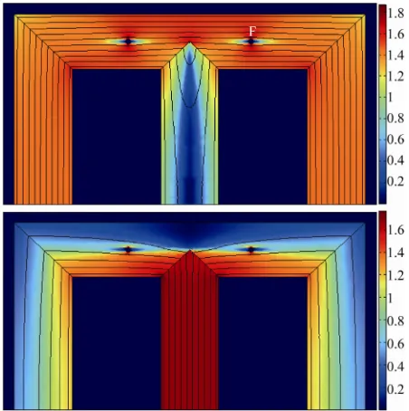
Due to presence of air gaps at the joints, magnetic flux travels between the overlapping laminations of yokes and limbs. When these laminations are saturated, flux crosses the air gaps [1]. This flux distortion causes additional localized losses. This additional loss cannot be evaluated from XY-plane models. Therefore Z-plane model is util-ized to solve this problem taking into account air gap at the joints [1,16,20,21]. In Figure 4, the magnetic flux density behavior for Single Step Lap (SSL) and Multi- Step Lap (MSL) structures are shown using CRGO steel while operating under a magnetic flux density of 1.7 Tesla.
0 2.5 5 7.5 10 12.5 15 17.5 20 -2
-1 0 1 2
Time [ms]
M
a
g
n
etic Flux
D
ensity [T]
data1 data2 Rolling Direction Cross-Rolling Direction
Figure 3. Magnetic flux density waveform at point P indi-cated in Figure 2.
Figure 4. Magnetic flux distribution at area of joints due to presence of air gaps while operating under magnetic flux density of 1.7 Tesla in CRGO steel, a) Single Step Lap, b) Multi-Step Lap.
The variation of magnetic flux density in the SSL and MSL joints along the line L, in Figure 4, is plotted and shown in Figure 5. As it is shown in Figure 5, the flux distortion takes place only in a distance of a few centi-meters around the air gaps. Therefore the application of z-plane model is limited to this area and it is independent of the overall structure of the transformer core [16].
For several magnetic flux densities, 2-D structure of
Figure 4 is solved and the extra localized joint loss is calculated. By integrating losses over the sheets and di-viding by thickness of sheets, ALJLden (W/m2) is
ob-tained [14,17]. By multiplying ALJLden and surface of
joints, total additional localized joint losses can be obtained [14].
2.3. Core Loss Model for Non-Sinusoidal Waveforms
As shown in Figure 3, the instantaneous magnetic flux densitywaveforms in the elements of transformer core demonstrate a non-sinusoidal variation. Therefore, in this
2 3 4 5 6 7 8 9
0 0.5 1 1.5 2 2.5
2 3 4 5 6 7 8 9
0 0.5 1 1.5 2 2.5
M
agne
ti
c f
lux de
ns
it
y [
T
]
Sheet Length [cm]
b) a)
Figure 5. Magnetic flux density along line L from Figure 4, (a) SSL structure; (b) MSL structure.
modeling the equations related to the sinusoidal wave- forms cannot be used.In recent years, accurate equations are developed to model the core loss when a non-sinu- soidal flux density waveform exists in the magnetic ma-terials. In this paper Equation (5) is used to calculate the losses in each element of the transformer core as pro- posed by [22,23]:
2
2 20 1.5 0
1 d
d
12 d
1 d
d . d
a m b m c T
n B n B n
h m t
T exc t
a B
P K B t
T t
B
K t
T t
(5)
where Bm, a, σ, ρ and T represent maximum flux density,
the sheet thickness, its conductivity, its mass density and the time period respectively. Kh, Kexc and na,b,care the
constant coefficients of the magnetic material. These coefficients can be obtained using the nominal loss of the magnetic sheets in specific frequencies and specific magnetic flux densities.
Using Equation (5), spatial distribution of core loss of XY-plane is shown in Figure 6. Stacking holes are ig-nored in Figure 6 for a better visualization.
3. Combination of Empirical and Numerical
Methods
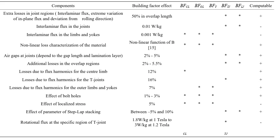
Empirical methods predict no-load loss based on building factor estimation. No-load loss and consequently BF con- sist of various parts. Reference [5] has categorized dif- ferent parts of BF and effect of each part by numerous experimental researches as indicated in Table 1.
Table 1. Components contributing the building factor [5].
Computable
BFLJ
BFTJ
BFY
BFOL
BFCL
Building factor effect Components
+ *
* 50% in overlap length
Extra losses in joint regions ( Interlaminar flux, extreme variation of in-plane flux and deviation from rolling direction)
- *
* 0.01 W/kg
Interlaminar flux in the joints
- *
* * 0.001 W/kg
Interlaminar flux in the limbs and yokes
+ *
* * Non-linear function of B
[15] Non-linear loss characterization of the material
+ *
* 2% - 5%
Air gaps at joints (depend to the gap length and lamination layer)
+ *
* 2% - 5.5%
Additional losses in the overlap regions
+ *
12% Losses due to flux harmonics for the centre limb
+ *
16% Losses due to flux harmonics for the T-joints
+ *
* 7%
Losses due to flux harmonics for the outer limbs and yokes
+ *
* * 1% - 3%
Effect of bolt holes
- *
* * 5%
Effect of localized stress
+ *
* Between –5% and 10%
Effect of parameter of Step-Lap stacking
- *
1.8W/kg at 1 Tesla to 3W/kg at 1.2 Tesla Rotational flux at the specific region of T-joint
TJ CL
Figure 6. Spatial distribution of core loss of XY-plane model in upper half of 3-phase 3-limb core.
factor [24]. General equation which is proposed by empi- rical methods can be written as follows:
. .
, , , , , ,
m yol m yol cl m cl
Lj m Lj Tj m Tj
CL SL B BF B V BF B V
BF B G N OL V BF B G N OL V (6)
where CL is predicted core losses. G, OL and N are air gap length, overlap distance and number of steps at joints respectively. SL is nominal loss of magnetic sheets. Vyol,
BFyol, Vcl, BFcl, VLj, BFLj, VTj and BFTj are volumes and
building factors of yokes and outer limbs, center limb, L-joints and T-joints respectively. Reference [5] has con-sidered volume of joints as overlap volume plus 15 mil-limeters of adjacent volume of core.
Some parts of different BFs shown in Table 1 can be calculated by numerical method introduced in Section 2. These computable parts are indicated by ‘+’ sign in Ta-ble 1. By elimination of these parts and inserting of
cal-culated losses through Equation (6), this equation can be rewritten as follows:
% % % %
, ,
yl yol cl Lj Lj Tj Tj
CL SL W
BF V V BF V BF V
XYL ZL G N OL
(7) where W is the total weight of core. XYL and ZL are losses computed form XY-plane model and Z-plane model. As shown in Table 1, by elimination of comput-able parts from Equation (6), other parts are common between yokes and limbs. Therefore, BFyl is introduced
as building factor of all limbs and yokes. Signs of ‘%’ indicate ratio of the part volume to the overall core vol-ume.
As mentioned before, SL·W is nominal loss of trans-former core (NL) that can be predicted by Epstein coeffi-cient. Also, in common designs of power transformer core such as mitred 45˚, the ratio of %VLj to %VTj is
con-stant. Therefore Equation (7) can be rewritten finally by these simplifications as follows:
, ,
% %
yl yl j j
ZL G N OL
CL NL BF V BF V
NL XYL
(8)
where %Vyl and BFylare percent volume and building
factor of yokes and limbs. %Vjand BFj are percent
[image:5.595.61.287.354.461.2]Variables of Equation (8) are G, BFyl and BFj. These
variables should be set by experimental data obtained from manufactured cores. Other parameters of Equation (8) can be either calculated in Section 2 or obtained us-ing geometrical data of core design.
4. Building Factor Optimization
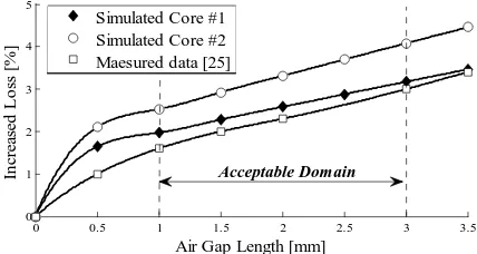
As shown in Section 3, after calculation of XY-plane losses and Z-plane losses with numerical methods, an optimization for selection of building factor (BF) and air gap length (G) is needed. First of all, relation between ZL and G should be determined. Figure 7 shows variation of ZL/NL versus G for various transformers for two exam-ple cores and a measured data from [25]. It can be seen in [25] that there is a linear relationship between ZL/NL
and G in the desired range where G varies from 1 to 3
millimeters. This is the result of an experimental meas-urement. Simulation results indicate the same thing (Figure 7). Therefore, ZL/NL can be written as follows:
ZL aG b
NL (9) where a and b are constant variables obtained by curve fitting. As illustrated in Figure 7, these parameters differ for various cores. Using Equations (9) and (8) can be rewritten as follows:
% %
yl yl j j
CL NL BF V BF V aG b XYL (10)
Assume the method has been provided by n number of transformer core design and measured no-load loss of them. The objective function of optimization is defined as summation of square of relative errors:
2 2 1 1 n n i i i
i i i
M CL OF Error M
4 i (11)where Mi is the measured core loss of ith transformer.
According to Equation (10), the objective function can be written as follows:
21 2 3
1
n i i i yl j
i
OF A BF A BF A G A (12)
where:
1
%
i yli
i
i
NL V
A
M (13)
2
%
i i
i i NL V A M j (14) 3 i i i a A M
(15)
4
i i i i
i
M b XYL
A
M
(16)
0 0.5 1 1.5 2 2.5 3 3.5 0 1 2 3 4 5
Air Gap Length [mm]
In cr eas ed Los s [% ] data5
Simulated Core #1 Simulated Core #2 Maesured data [25]
[image:6.595.314.528.90.204.2]Acceptable Domain
Figure 7. Percentage increases of power losses as a function of air gap length.
By some mathematical works, Equation (12) can be written as a standard Quadratic Programming equation as follows [26]:
21 1 2 1 3
1 1 1
2
1 2 2 2 3
1 1 1
2
1 3 2 3 3
1 1 1
2
1 4 2 4 3 4 4
1 1 1 1
2.
n n n
i i i i i
i i i
n n n
T
i i i i i
i i i
n n n
i i i i i
i i i
n n n n
T
i i i i i i i
i i i i
yl j
A A A A A
OF x A A A A A x
A A A A A
A A A A A A x A
x BF BF G
(17) The last term in Equation (17) is a constant value and can be eliminated from the objective function. Finally, the QP problem is written as follows:min
subject to: 1 mm 3 mm
0 ,
yl j
OF G BF BF
(18)
Considering the variance definition, the objective function can be assumed equal to Equation (19):
2min var( )
subject to: 1 mm 3 mm
0 ,
yl j
Error Error
G BF BF
(19)
where Error is average of relative errors and var(Error) indicates variance of them.
By solving QP [26], the best possible solution for building factors is obtained. Also, a good estimation for air gap average length which is inevitable in manufac-turing of core is attained. These parameters minimize average and standard deviation of prediction error as much as possible. As shown in Figure 8, by using XYL
-12 -10 -8 -6 -4 -2 0 2 4 6 8 0
0.02 0.04 0.06 0.08 0.1 0.12 0.14 0.16
Deviation [%]
P
ro
b
ab
ili
ty
XYL XYL + ZL Predicted Loss
Figure 8. Probability distributions of estimated core losses by and without using building factors optimization.
estimation has a bias error and undesired standard devia- tion. By introducing losses due to joints as ZL in predic- tion, average error reduces slightly but standard devia- tion does not change considerably. Finally by consider- ing corrective building factors the core loss estimation becomes reasonable and average error and standard deviation reduce to an acceptable range. Also these opti- mized parameters can be used for core loss estimation of upcoming designs and can be improved every time required by new measured data. Therefore, the factory can use its personalized data to improve the no-load loss prediction without changing complex numerical program, only by a simple optimization using measured data.
5. Verification of The Proposed Method
5.1. Verification with Literature
Different parts of the proposed method can be verified against the published works in the related literature. For example, Figure 3 and Figure 6 demonstrate a very good similarity with the results in [1]. Also Figure 4 and
Figure 5 are verified with the results of [16] when CRGO steel is used.
5.2. Verification with Constructed Cores
Reference [27] reported complete data of a constructed core and measured core loss. This core is made of CRGO (grade M5) and by mitred 45˚ joints. The overlap length on joints is 5 mm, the core has one pocket by width of 70 mm, height and length of core are 300 mm and 350 mm. Core losses measured by a well-designed circuit and ex- isting building factor over different flux densities is re- ported to have tolerance of 4%. As shown in Figure 9, estimation has a significant error by using only XY-plane losses for loss prediction. As mentioned in [27], air gap length (G) is tried to be less than 1 mm. Figure 9 indi- cates that even with assuming 1 mm air gap, estimated loss is less than the measured data. However, by intro- ducing corrective building factor equal to 0.09, all pre-
1.5 1.55 1.6 1.65 1.7 1.75 1.8 1.85 1
1.05 1.1 1.15 1.2 1.25 1.3 1.35 1.4
Flux Density [T]
B
u
ld
in
g
F
ac
to
r
XYL XYL + ZL Peridected Loss Measured Loss [2]
Figure 9. Predicted core losses by and without using build-ing factors optimization at different flux densities.
dicted losses will come in the expected range. Measured data has an error of 4% which is recognized by [27] as measuring circuit error. This case can show that numeri-cal methods separately cannot model transformer core loss, when real air gap length is used. Although by using greater air gap this weakness can be solved for numerical methods, but transformer design programs will use in-correct estimation about importance of air gap joints.
5.3. Verification with Full-Size Transformers
The authors had opportunity to use 54 full size trans-formers of one company for verification of the proposed method. These transformers are of 12 different designs. For every type of design four or five manufactured transformers have been tested and the mean of their core losses has been nominated for its design. All transform-ers are made of cold rolled grain oriented (M5T30) ma-terial. The cores were three phase three limb stacked core with structures of mitred 45˚. Multi-Step lap joints have been designed for all cases. From these 12 different types, eight types have been used for training of method and computing of building factors and air gap length. Four types have been used for testing the proposed method named as the test group here. Optimization shows that the best value of building factors for joints is 37.01% and its best value for yokes and limbs is 0.21%.
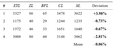
Also, the mean air gap length for the studied trans- formers of that company is 3 millimeters. By these pa- rameters, the predicted core losses for the test group are shown in Table 2. As it can be seen in Table 2, this hy- brid combination of numerical and empirical methods has an excellent ability to estimate core losses of trans- formers.
6. Summery and Conclusions
Table 2. Tested results (all losses per Watt).
# XYL ZL BFL CL Mi Deviation
1 3327 86 65 3478 3622 +3.98%
2 1175 40 29 1244 1235 –0.73%
3 1572 46 33 1651 1640 –0.67%
4 3008 80 60 3148 3062 –2.81%
Mean –0.06%
core distribution transformers. Empirical methods can model all components of no-load loss while numerical methods are able to analyze different parameters accu- rately. In the proposed method, first all of the comput- able parts of building factor are calculated by FEM mo- dels, and then other components of BF are optimized by quadratic programming. If more measured data become available, the core loss estimation is possible to be im- proved over time by using this method. Meanwhile, dif-ferent companies can obtain difdif-ferent results for the same designs and materials employed, based on their historical data.
In the future work, the authors will use magnetizing current for estimation of the effective air gap length and will improve the method by introducing an accurate mea- sured air gap length.
REFERENCES
[1] G. F. Mechler and R. S. Girgis, “Calculation of Spatial Loss Distribution in Stacked Power and Distribution Transformer Cores,” IEEE Transactions on Power De-livery, Vol. 13, No. 2, 1998, pp. 532-537.
doi:10.1109/61.660925
[2] P. S. Georgilakis, “Spotlight on Modern Transformer Design,” Springer-Verlag, New York, 2009.
doi:10.1007/978-1-84882-667-0
[3] NEMA Standard TP 1, Guide for Determining Energy Efficiency for Distribution Transformers, 2002.
[4] CENELEC Standards HD 428.1, Three Phase Oil-im-mersed Distribution Transformers 50 Hz, from 50 kVA to 2500 kVA, with Highest Voltage for Equipment Not Ex-ceeding 36 kV, 1992.
[5] A. J. Moses, “Prediction of Core Losses of Three Phase Transformers from Estimation of the components Con-tributing to the Building Factor,” Journal of Magnetism and Magnetic Materials, Vol. 254-255, 2003, pp. 615- 617. doi:10.1016/S0304-8853(02)00911-3
[6] A. Basak and, A. A. Bonyar, “Effects of transformer core assembly on building factors,” Journal of Magnetism and Magnetic Materials, Vol. 112, No. 1-3, 1992, pp. 406- 408. doi:10.1016/0304-8853(92)91214-E
[7] K. A. L. Abdul-Retha and A. Basak, “A Comparison of Building Factors for Different Types of Transformer Cores Built With Highly Oriented and Conventional
Grade Silicon-Iron Laminations,” Journal of Magnetism and Magnetic Materials, Vol. 26, No. 1-3, 1982, pp. 92- 94. doi:10.1016/0304-8853(82)90123-8
[8] Z. Valkovic, “Additional Losses in Three-Phase Trans-former Cores,” Journal of Magnetism and Magnetic Ma-terials, Vol. 41, No. 1-3, 1984, pp. 424-426.
doi:10.1016/0304-8853(84)90237-3
[9] G. W. Swift, “Excitation current and Power Loss Char-acteristics for Mitered Joint Power Transformer Cores,” IEEE Transactions on Magnetic, Vol. 11, No. 1, 1975, pp. 61-64. doi:10.1109/TMAG.1975.1058541
[10] M. Elleuch and M. Poloujadoff, “New Transformer Model Including Joint Air Gaps and Lamination Anisot-ropy,” IEEE Transactions on Magnetic, Vol. 34, No. 5, 1998, pp. 3701-3711. doi:10.1109/20.718532
[11] M. Elleuch, M. Poloujadoff, “Analytical model of iron losses in power transformers,” IEEE Transactions on Magnetic, Vol. 39, No. 2, 2003, pp. 973-980.
doi:10.1109/TMAG.2003.808591
[12] C. Nussbaum, T. Booth, A. Ilo and H. Pfutzner, “A Neu-ral Network for the Prediction of Performance Parameters of Transformer Cores,” Journal of Magnetism and Mag-netic Materials, Vol. 160, No. 1, 1996, pp. 81-83. doi:10.1016/0304-8853(96)00122-9
[13] C. Nussbaum, H. Pfutzner, Th. Booth, N. Baumgartinger, A. Ilo and M. Clabian, “Neural Networks for the Predic-tion of Magnetic Transformer Core Characteristics,” IEEE Transactions on Magnetic, Vol. 36, No. 1, 2000, pp. 313-329. doi:10.1109/20.822542
[14] E. Hajipour, M. Vakilian and S. A. Mousavi, “A Novel Fast FEA No-Load Loss Calculation Method for Stacked Core Three Phase Distribution Transformers,” 45th In-ternational Universities Power Engineering Conference, Cardiff, 2010, unpublished.
[15] R. Prieto, J. A. Cobos, V. Bataller, O. Garcia and J. Ucedci, “Study of Toroidal Transformers by Means of 2D Approaches,” Proceeding of 28th IEEE Annual Power Electronics Specialists Conference, St. Louis, 22-27 June 1997, pp. 621-626.
[16] G. F. Mechler and R. S. Girgis, “Magnetic Flux Distribu-tion in Transformer Core Joints,” IEEE TransacDistribu-tions on Power Delivery, Vol. 15, No. 1, 2000, pp. 198-203. doi:10.1109/61.847251
[17] E. G. teNyenhuis, R. S. Girgis and G. F. Mechler, “Other Factors Contributing to the Core Loss Performance of Power and Distribution Transformers,” IEEE Transac-tions on Power Delivery, Vol. 16, No. 4, 2001, pp. 648- 653. doi:10.1109/61.956752
[18] NEMA Standard TP 2, Standard Test Method for Meas-uring the Energy Consumption of Distribution Trans-formers, 2005.
[19] M. Enokizono and N. Soda, “Finite Element Analysis of Transformer Model Core with Measured Reluctivity Tensor,” Transactions on Magnetic, Vol. 33, No. 5, 1997, pp. 4110-4112.
[24] A. J. Moses, “Comparison of Transformer Loss Predic-tion from Computed and Measured Flux Density Distri-bution,” IEEE Transactions on Magnetic, Vol. 34, No. 4, 1998, pp. 1186-1188. doi:10.1109/20.706473
Key Quantity for the Optimization of Transformer Core Operation,” Journal of Magnetism and Magnetic Materi-als, Vols. 215-216, No. 1, 2000, pp. 637-640.
doi:10.1016/S0304-8853(00)00248-1
[25] F. Loffer, T. Booth, H. Pfutzner, C. Bengtsson and K. Gram, “Relevance of Step-Lap Joints for Magnetic Characteristics of Transformer Cores,” IEE Proceeding in Electric Power Application, Vol. 142, No. 6, 1995, pp. 371-378.doi:10.1049/ip-epa:19952228
[21] J. C. Olivares, Y. Liu, J. Canedo, R. Escarela-Perez, J. Driesen and P. Moreno, “Reducing Losses in Distribution Transformers,” IEEE Transactions on Power Delivery, Vol. 18, No. 4, 2003, pp. 821-826.
doi:10.1109/TPWRD.2003.813851
[26] M. R. Pishvaie, “Process Optimization Course” 2010. http://sharif.ir/~pishvaie/OptimCoursePage.htm. [22] S. A. Mousavi, “Harmonic Core Losses Calculation in
Power Transformers,” M.Sc. Thesis, University of
Te-hran, TeTe-hran, 2008. [27] Z. Valkovic, “Influence of Transformer Core Design on Power Losses,” IEEE Transactions on magnetic, Vol. 18, No. 2, 1982, pp. 801-804.
doi:10.1109/TMAG.1982.1061824 [23] W. A. Roshen, “A Practical, Accurate and Very General