ISSN Online: 2161-4725 ISSN Print: 2161-4717
DOI: 10.4236/ijaa.2018.84028 Dec. 29, 2018 406 International Journal of Astronomy and Astrophysics
Artificial Equilibrium Points in the Low-Thrust
Restricted Three-Body Problem When Both the
Primaries Are Oblate Spheroids
Amit Mittal
1, Krishan Pal
21Department of Mathematics, A.R.S.D College, University of Delhi, New Delhi, India
2Department of Mathematics, Maharaja Agrasen College, University of Delhi, New Delhi, India
Abstract
This paper studies the existence and stability of the artificial equilibrium points (AEPs) in the low-thrust restricted three-body problem when both the primaries are oblate spheroids. The artificial equilibrium points (AEPs) are generated by canceling the gravitational and centrifugal forces with conti-nuous low-thrust at a non-equilibrium point. Some graphical investigations are shown for the effects of the relative parameters which characterized the locations of the AEPs. Also, the numerical values of AEPs have been calcu-lated. The positions of these AEPs will depend not only also on magnitude and directions of low-thrust acceleration. The linear stability of the AEPs has been investigated. We have determined the stability regions in the xy, xz and yz-planes and studied the effect of oblateness parameters A1
(
0<A1<1)
and(
)
2 0 2 1
A <A < on the motion of the spacecraft. We have found that the
sta-bility regions reduce around both the primaries for the increasing values of oblateness of the primaries. Finally, we have plotted the zero velocity curves to determine the possible regions of motion of the spacecraft.
Keywords
Restricted Three-Body Problem, Artificial Equilibrium Points, Low-Thrust, Stability, Oblate Spheroid, Zero Velocity Curves
1. Introduction
Generally, the restricted three-body problem is one of the most important problem in the field of celestial mechanics. In the Restricted Three-Body Problem (R3BP), the mass of the third body (i.e., the spacecraft) is assumed to be
How to cite this paper: Mittal, A. and Pal, K. (2018) Artificial Equilibrium Points in the Low-Thrust Restricted Three-Body Problem When Both the Primaries Are Oblate Spheroids. International Journal of Astronomy and Astrophysics, 8, 406-424.
https://doi.org/10.4236/ijaa.2018.84028 Received: November 2, 2018
Accepted: December 26, 2018 Published: December 29, 2018 Copyright © 2018 by authors and Scientific Research Publishing Inc. This work is licensed under the Creative Commons Attribution International License (CC BY 4.0).
http://creativecommons.org/licenses/by/4.0/
DOI: 10.4236/ijaa.2018.84028 407 International Journal of Astronomy and Astrophysics
negligible in comparison to the two more massive bodies, defined as the primary and the secondary. It is assumed that the two primaries revolving in circular orbits about their common center of mass, known as the barycenter. It is then possible to model the motion of the spacecraft in a frame of reference that rotates about the barycenter at the same rotation rate as the two primaries. The motion of the spacecraft is affected by the motion of the primaries but not affect them. To study the motion of the third body is known as restricted three-body problem. There are five equilibrium points in the classical restricted three-body problem (R3BP), three of them are on the straight line joining the primaries, called collinear equilibrium points, and two of them setup equilateral triangle with the primaries. The collinear equilibrium points L1,2,3 are always unstable in the linear sense for any value of mass parameter µ whereas the triangular points L4,5 are stable if µ µ< c=0.03852. Szebehely [1]. Many perturbing
forces, like oblateness, radiation forces of the primaries, Coriolis and centrifugal forces etc., have been included in the study of the R3BP. Many results have been published to the study in the restricted three-body problem with effect of oblateness; see Subbarao and Sharma [2], Bhatnagar and Chawla [3], Tsirogiannis et al. [4], Mittal et al. [5], Singh [6], Beevi and Sharma [7], Abouelmagd [8], Jain and Aggarwal [9]. Zotos [10] has determined the basins of attraction associated with the equilibrium points in the planar CR3BP where one of the primary bodies is an oblate spheroid or an emitter of radiation. Also, he has noticed that the structure of the basins of convergence is more affected by the mass ratio and radiation pressure parameters than the oblateness parameter. Srivastava et al. [11]
have introduced Kustaanheimo-Stiefel (KS)-transformation to reduce the order of singularities arising due to the motion of an infinitesimal body in the vicinity of smaller primary in the R3BP when the bigger primary is a source of radiation and smaller one as an oblate spheroid. They have found that KS-regularization reduces the order of the pole from five to three at the point of singularity of the governing equations of motion.
The new equilibrium points can be generated if the continuous constant acceleration uses by a spacecraft to balance the gravitational and centrifugal forces. These points are usually referred to Artificial Equilibrium Points (AEPs). Recently, low-thrust propulsion systems as solar-sail and the electric propulsion are being developed not only for controlling satellite orbit, but also as main engines for interplanetary transfer orbits. These low-thrust propulsion systems are able to provide continuous control acceleration to the spacecraft and thus, increase mission design flexibility. Farquhar [12] has studied the concept of telecommunication systems using equilibrium points and investigated ballistic periodic orbits about these points in the Earth-Moon system. Dusek [13], McInnes et al. [14], Broschart and Scheeres [15] have studied the stability of equilibrium points with continuous control acceleration. Morimoto et al. [16]
DOI: 10.4236/ijaa.2018.84028 408 International Journal of Astronomy and Astrophysics
have investigated the artificial three-body equilibria for hybrid low-thrust propulsion. In their study, they have introduced a new concept of creating AEPs in the R3BP when the third body uses a hybrid of solar-sail and electric propulsion. Further, there are many precise work related to the low-thrust restricted three-body problem; see Bombardelli and Pelaez [18], Aliasi et al.[19] [20], Ranjana and Kumar [21], Yang et al. [22], Lei and Xu [23]. Bu et al.[24]
have investigated the positions and dynamical characteristic of AEPs in a binary asteroid system with continuous low-thrust. They have found the stable regions of AEPs by a parametric analysis and studied the effect of the mass ratio and ellipsoid parameters on the stable region. Further, they have analyzed the effect of the continuous low-thrust on the feasible region of motion by ZVCs.
In the present work, we have focussed on the study of the motion of the spacecraft in the low-thrust restricted three-body problem when both the primaries are oblate spheroids. Here, we have extended the work of Morimoto et al. [16]. We have arranged the present work as follows: In Secttion 2, we have derived the equations of motion of the spacecraft. In Secttion 3, we have found the locations of the AEPs. In Secttion 4, we have determined the linear stability. In Secttion 5, we have computed the zero velocity curves. Finally, in Secttion 6, we have concluded the results obtained.
2. Equations of Motion
In this section, we shall determine the equations of motion of the spacecraft in the low-thrust restricted three-body problem when both the primaries are oblate spheroids. Suppose two bodies of masses m1 and m2
(
m m1 > 2)
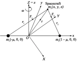
are the primaries moving with angular velocity ω in circular orbits about their centerof mass O taken as origin, and let the infinitesimal body (spacecraft) of mass m3 be also moving in the plane of motion of m1 and m2. The motion of the spacecraft is affected by the motion of m1 and m2 but not affect them. The line joining the primaries m1 and m2 is taken as X-axis and the line passes through the origin O and perpendicular to the X-axis and lying in the plane of motion of m1 and m2 is considered as Y-axis, the line which passes through the origin and perpendicular to the plane of motion of the primaries is taken as Z-axis. In a synodic frame, the system of synodic coordinates O xyz
( )
, initially coincident with the system of inertial coordinates O XYZ(
)
, rotating with the angular velocity ω about Z-axis; (the z axis is coincident with Z-axis). Let the primaries of masses m1 and m2 be located at(
−µ
,0,0)
and(
1−µ
,0,0)
respectively and the spacecraft be located at the point(
x y z, ,)
(see Figure 1). The angular velocity of the primaries is given by the relation(
1 2)
3
G m m l
ω= + , where l is
distance between the primaries, and G is Gravitational constant. We scale the units by taking the sum of the masses and the distance between the primaries both equal to unity. Therefore m1= −1 µ, m2 =µ and 2
1 2
m m m µ =
DOI: 10.4236/ijaa.2018.84028 409 International Journal of Astronomy and Astrophysics
Figure 1. Configuration of the problem.
1 2 1
m m+ = . Also, the scale of the time is chosen so that the gravitational
constant is unity. Let a b c1, ,1 1 and a b c2, ,2 2 are the semi axes of rigid bodies of masses m1 and m2 respectively. The equation of motion of the spacecraft in vector form is expressed as
2
2
d 2 d ,
d
dt + × t = − ∇Ω =
r w r a F (1)
where Ω is the potential (McCuskey [25]) of the system that combines the gravitational potential and the potential from the centripetal acceleration which is defined as
(
)
(
)
2
1
2 2 2
3 3
1 2 1 2
1
1 ,
2 2 2
A A
n x y
r r r r
µ µ
µ µ −
−
Ω = − + − − − −
and
F = total force acting on m3 = F F1+ 2, 1
F = Gravitational force exerted on m3 due to m1 along m3m1, 2
F = Gravitational force exerted on m3 due to m2 along m3m2.
The vector a=
(
a a ax, ,y z)
is low-thrust acceleration and r=(
x y z, ,)
T isthe position vector of the spacecraft from the origin. Thus, the equations of motion of the spacecraft with continuous low-thrust in dimensionless co-ordinate system can be written as Morimoto et al. [16]
* * * 2 , 2 , ,
x x x
y y y
z z z
x ny a
y nx a
z a
− = −Ω + = −Ω
+ = −Ω + = −Ω
= −Ω + = −Ω
(2)
where Ω* is the effective potential of the system with continuous low-thrust can be written as
(
)
(
)
*
2
1
2 2 2
3 3
1 2 1 2
1
1 ,
2 2 2
x y z
x y z
a x a y a z
A A
n x y a x a y a z
r r r r
µ µ
µ µ
Ω = Ω − − −
− −
= − + − − − − − − −
where
(
)
2 2 21 ,
r = x+µ +y +z
(
)
2 2 22 1 ,
DOI: 10.4236/ijaa.2018.84028 410 International Journal of Astronomy and Astrophysics
2 2 2.
x y z
a= a a a+ +
The required mean motion of the primaries denoted by n, which is given by the relation:
(
)
2 1 2 3 1 , 2n = + A A+
where A1 is the oblateness parameter of m1 which is defined as
(
)
2 2
1 1
1 52 ,0 1 1, 1 1 1 1
a c
A A a b a c
l −
= < < = > , and A2 is the oblateness parameter of m2
which is also defined as 22 22
(
)
2 52 ,0 2 1, 2 2 2 2
a c
A A a b a c
l −
= < < = > , where l be the
distance between the primaries.
3. Locations of the Artificial Equilibrium Points
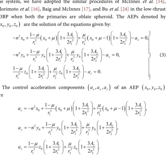
In order to find the AEPs of the system, taking velocity and acceleration of the system equal to zero. For obtaining the artificial equilibrium points (AEPs) of the system, we have adopted the similar procedures of McInnes et al. [14], Morimoto et al. [16], Baig and McInnes [17], and Bu et al. [24] in the low-thrust R3BP when both the primaries are oblate spheroid. The AEPs denoted by
(
x y z0, ,0 0)
are the solution of the equations given by:(
)
(
)
2 1 2
0 3 0 2 3 0 2
1 1 2 2
2 1 2
0 3 0 2 3 0 2
1 1 2 2
1 2
0 0
3 2 3 2
1 1 2 2
3 3
1 1 1 1 0,
2 2
3 3
1 1 1 0,
2 2
3 3
1 1 1 0.
2 2
x
y
z
A A
n x x x a
r r r r
A A
n y y y a
r r r r
A A
z z a
r r r r
µ µ µ µ
µ µ µ µ − − + + + + + − + − = − − + + + + − = − + + + − = (3)
The control acceleration components
(
a a ax, ,y z)
of an AEP(
x y z0, ,0 0)
are(
)
(
)
2 1 1
0 3 0 2 3 0 2
1 1 2 2
3 3
1 1 1 1 ,
2 2
x A A
a n x x x
r r r r
µ
µ
µ
µ
−
= − + + + + + − +
2 1 2
0 3 0 2 3 0 2
1 1 2 2
3 3
1 1 1 ,
2 2
y A A
a n y y y
r r r r
µ
µ
−
= − + + + +
1 2
0 0
3 2 3 2
1 1 2 2
3 3
1 1 1 .
2 2
z A A
a z z
r r r r
µ
µ
−
= + + +
When A1=0,A2=0,a=
(
0,0,0)
, the above Equations (3) reduce to the clas- sical equations obtained by Szebhely [1]. When A1=A2=0 and a≠(
0,0,0)
, the above Equations (3) reduce to the equations obtained by Morimoto et al.[16]. Solving Equations (3) for z=0, then the AEPs are lie in the xy-plane and
obtained by solving * 0, * 0
x y
Ω = Ω = . We have obtained the five AEPs for given
[image:5.595.213.541.312.620.2]thrust and oblateness parameters denoted by L L L L1, , ,2 3 4 and L5 as shown in
DOI: 10.4236/ijaa.2018.84028 411 International Journal of Astronomy and Astrophysics
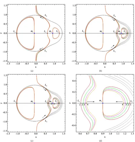
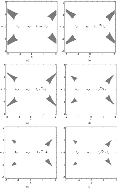
Figure 2. The locations of the five AEPs in the low-thrust R3BP with the effect of constant control acceleration and oblateness parameters. Panel-(a) for µ=0.1, A1=0.0015, A2=0.0015 and for different values of a=
(
0.0001,0,0 gray,red)(
)
,(
0.01,0,0 gray,green)(
)
,(
0.02,0,0 gray,magenta)(
)
,(
0.03,0,0 gray,orange)(
)
, and panel-(b) for µ=0.1, A1=0.0015,(
0.0001,0,0)
=
a and for different values of A2=0.0015 gray,red
(
)
, 0.15 gray,green(
)
, 0.35 gray,magenta(
)
,(
)
0.55 gray,orange , panel-(c) for µ=0.1, A2=0.0015, a=
(
0.0001,0,0)
and for different values of A1=0.0015 gray,red(
)
,(
)
0.15 gray,green , 0.35 gray,magenta
(
)
, 0.55 gray,orange(
)
, panel-(d) shows the zoomed part of panel-(c) near the primary m2.From Figure 2(a), we have observed that when a=
(
ax,0,0)
is increasing,DOI: 10.4236/ijaa.2018.84028 412 International Journal of Astronomy and Astrophysics
the AEP L2 is shifted from left to right away from the primary m2, the AEP L3 is shifted from left to right towards the bigger primary m1, and the AEPs L4 and L5 move towards the x-axis.
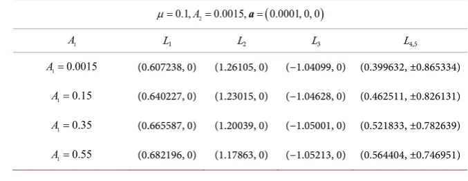
[image:7.595.210.539.300.415.2]From Figure 2, panel-c, we have observed that when A1 is increasing, the AEP L1 is shifted from left to right towards the primary m2, the AEP L2 is shifted from right to left towards the primary m2, the AEP L3 has almost negligible movement, and the AEPs L4 and L5 move towards the x-axis. In addition, we have calculated the numerical values of the AEPs and shown in Tables 1-3. We have observed that there exist three collinear and two non-collinear AEPs. Further, we have observed that the AEPs L4 and L5 are symmetric about the x-axis. Also, it is observed that the AEPs are the new positions of equilibrium points with the effect of continuous low-thrust and oblateness parameters which are different from the natural equilibrium points.
Table 1. The AEPs in the xy-plane when a is varying.
1 2
0.1,A 0.0015,A 0.0015
µ= = =
a L1 L2 L3 L4,5
(
0.0001,0,0)
=
a (0.607238, 0) (1.26105, 0) (−1.04099, 0) (0.399632, ±0.865334)
(
0.01,0,0)
=
a (0.606555, 0) (1.25943, 0) (−1.04409, 0) (0.360261, ±0.882827)
(
0.02,0,0)
=
a (0.605864, 0) (1.25783, 0) (−1.04724, 0) (0.313254, ±0.901830)
(
0.03,0,0)
=
[image:7.595.211.539.452.567.2]a (0.605170, 0) (1.25623, 0) (−1.05042, 0) (0.256260, ±0.922021)
Table 2. The AEPs in the xy-plane when A2 is varying.
(
)
1
0.1,A 0.0015, 0.0001, 0, 0
µ= = a=
2
A L1 L2 L3 L4,5
2 0.0015
A = (0.607238, 0) (1.26105, 0) (−1.040990, 0) (0.399632, ±0.865334)
2 0.15
A = (0.517691, 0) (1.33070, 0) (−0.978206, 0) (0.337489, ±0.826131)
2 0.35
A = (0.469823, 0) (1.35936, 0) (−0.914454, 0) (0.278167, ±0.782639)
2 0.55
A = (0.439717, 0) (1.37309, 0) (−0.865643, 0) (0.235596, ±0.746951)
Table 3. The AEPs in the xy-plane when A1 is varying.
(
)
2
0.1,A 0.0015, 0.0001, 0, 0
µ= = a=
1
A L1 L2 L3 L4,5
1 0.0015
A = (0.607238, 0) (1.26105, 0) (−1.04099, 0) (0.399632, ±0.865334)
1 0.15
A= (0.640227, 0) (1.23015, 0) (−1.04628, 0) (0.462511, ±0.826131)
1 0.35
A= (0.665587, 0) (1.20039, 0) (−1.05001, 0) (0.521833, ±0.782639)
1 0.55
[image:7.595.200.539.602.733.2]DOI: 10.4236/ijaa.2018.84028 413 International Journal of Astronomy and Astrophysics
4. Stability of the Artificial Equilibrium Points
To determine the linear stability of the system of AEPs in the low-thrust R3BP when both the primaries are oblate spheroid. We have followed the linear stability procedure of Morimoto et al. [16]. Firstly, we have linearized the equations of motion of the spacecraft and then linear stability is studied. To establish the spacecraft at a non-equilibrium point, a continuous low-thrust is provided to the spacecraft. Now, giving the small displacement to
(
x y z0, ,0 0)
as x x= 0+δx,y y= 0+δy,z z= 0+δ δ δ δz,(
x, ,y z1)
. After using above displace-ments, the linearized equations corresponding to Equations (2) are given by
0 0 0
0 0 0
0 0 0
2 ,
2 ,
,
x y xx x xy y xz z
y x yx x yy y yz z
z zx x zy y zz z
n n
δ δ δ δ δ
δ δ δ δ δ
δ δ δ δ
− = Ω + Ω + Ω
+ = Ω + Ω + Ω
= Ω + Ω + Ω
(4)
where the superscript “0” in Equations (4) indicates that the values are to be calculated at the AEP
(
x y z0, ,0 0)
under consideration. The characteristic rootλ satisfies the given characteristic equation
( )
(
)
(
( ) ( ) ( )
)
( )
( )
( )
6 0 0 0 2 4 0 0 0 0 0 0
2 2 2
0 0 0 2 0 2 0 0 0
2 2 2
0 0 0 0 0 0 0 0 0
4
4
2 0.
xx yy zz xx yy xx zz yy zz
xy xz yz zz xx yy zz
xy xz yz xy zz xz yy yz xx
f n
n
λ λ λ
λ
= + Ω + Ω + Ω + + Ω Ω + Ω Ω + Ω Ω
− Ω − Ω − Ω + Ω + Ω Ω Ω
+ Ω Ω Ω − Ω Ω − Ω Ω − Ω Ω
=
(5)
If a characteristic root λ satisfies the Equation (5), then Equation (5) can be
rewritten as
(
)
(
( ) ( ) ( )
)
( )
( )
( )
6 0 0 0 2 4 0 0 0 0 0 0
2 2 2
0 0 0 2 0 2 0 0 0
2 2 2
0 0 0 0 0 0 0 0 0
4
4
2 0.
xx yy zz xx yy xx zz yy zz
xy xz yz zz xx yy zz
xy xz yz xy zz xz yy yz xx
n
n
λ λ
λ
+ Ω + Ω + Ω + + Ω Ω + Ω Ω + Ω Ω
− Ω − Ω − Ω + Ω + Ω Ω Ω
+ Ω Ω Ω − Ω Ω − Ω Ω − Ω Ω =
(6)
We see that all the powers of λ in Equation (6) are even numbers and Equation (6) be a six degree equation in λ. If k=λ2, then we get
(
) (
( ) ( ) ( )
)
( )
( )
( )
3 0 0 0 2 2 0 0 0 0 0 0
2 2 2
0 0 0 2 0 0 0 0
2 2 2
0 0 0 0 0 0 0 0 0
4
4
2 0.
xx yy zz xx yy xx zz yy zz
xy xz yz zz xx yy zz
xy xz yz xy zz xz yy yz xx
k n k
n k
+ Ω + Ω + Ω + + Ω Ω + Ω Ω + Ω Ω
− Ω − Ω − Ω + Ω + Ω Ω Ω
+ Ω Ω Ω − Ω Ω − Ω Ω − Ω Ω =
(7)
Equation (7) is a cubic equation in k and can be rewritten as
3 2
1 2 3 0,
k +d k +d k d+ = (8)
where
0 0 0 2
1 xx yy zz 4 ,
d = Ω + Ω + Ω + n
( ) ( ) ( )
2 2 20 0 0 0 0 0 0 0 0 2 0
2 xx yy xx zz yy zz xy xz yz 4 zz,
DOI: 10.4236/ijaa.2018.84028 414 International Journal of Astronomy and Astrophysics
( )
2( )
2( )
20 0 0 0 0 0 0 0 0 0 0 0
3 xx yy zz 2 xy xz yz xy zz xz yy yz xx,
d = Ω Ω Ω + Ω Ω Ω − Ω Ω − Ω Ω − Ω Ω
and d1, d2, and d3 are the real coefficients of k that depend on the second ordered derivatives of Ω with respect to x and y. Now, we determine the linear stability of the AEPs by finding the characteristic roots of Equation (8). We know that all the characteristic roots of a cubic equation are either real numbers or one of them is a real number and other characteristic roots are imaginary numbers. According to stability theory, a necessary and sufficient condition for an AEP to be linearly stable is that all the characteristic roots of Equation (5) lie in the left-hand side of the λ-plane (i.e., λ ≤0). If one or more characteristic roots of
Equation (5) lie in the right-hand side of the λ-plane, then the system of AEPs is always unstable. If all the characteristic roots of Equation (5) lie to the left-hand side of λ-plane, then Equation (8) must have three real and negative roots. The resulting linear stability conditions according to Morimoto et al. [16] and Descartes sign rule, the system of AEPs is linearly stable if and only if
1 2
0, 0, 0
D≥ d > d > and d3>0, where D is the discriminant of the cubic
Equation (8) and is given by:
2 3
3 2
1 1 2 1
3 2
2 9
1 1 .
4 27 27 3
d d d d
D= d + − + d −
(9)
It is concluded that the system of AEPs is linearly stable when D≥0,d1>0,
2 0
d > and d3 >0. Now, we have found the stability regions in the xy, xz and
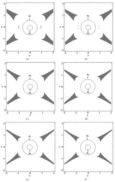
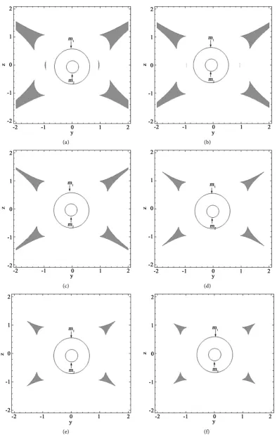
yz-planes as shown in Figures 3-8. In Figure 3, Figure 5, Figure 7, we have drawn the stability regions for the fixed values of µ =0.1, A1=0.0015 and for different values of oblateness parameter A2=0.0015,0.15,0.35,0.55,0.75,0.95. In Figure 4, we have plotted the stability regions for the fixed values of
µ
=0.1,2 0.0015
A = and for different values of oblateness parameter
1 0.0015,0.015,0.035,0.055,0.075,0.095
A = . In Figure 6 and Figure 8, we have
plotted the stability regions for the fixed values of
µ
=0.1, A2=0.0015 andfor different values of oblateness parameter A1=0.0015,0.15,0.35,0.55,0.75,0.95. From, Figures 3-8, we have observed that the stability regions decrease around both primaries for the increasing values of oblateness parameters A A1, 2∈
( )
0,1 and for fixed value of mass parameterµ
=0.1. Also, it is observed that theAEPs located in the stable regions are linearly stable otherwise unstable.
5. Zero Velocity Curves
In this section, we shall determine the possible regions of motion of the spacecraft in the low-thrust restricted thee-body problem when both the primaries are oblateness spheroid. The Jacobian Integral of the equations of motion (2) is defined as
(
2 2 2)
2 .
C= Ω + x +y +z (10)
DOI: 10.4236/ijaa.2018.84028 415 International Journal of Astronomy and Astrophysics
Figure 3. Stable regions (gray area) in the xy-plane for fixed values of µ=0.1, A1=0.0015 and for different values of oblateness parameter A2
(
0<A2<1)
(a) for A2=0.0015; (b) A2=0.15; (c) A2=0.35; (d) A2=0.55; (e) A2=0.75; (f)2 0.95
DOI: 10.4236/ijaa.2018.84028 416 International Journal of Astronomy and Astrophysics
Figure 4. Stable regions(gray area) in the xy-plane for µ=0.1, A2=0.0015 and for different values of oblateness parameter
(
)
1 0 1 1
DOI: 10.4236/ijaa.2018.84028 417 International Journal of Astronomy and Astrophysics
Figure 5. Stable regions (gray area) in the xz-plane for µ=0.1, A1=0.0015 and for different values of oblateness parameter
(
)
2 0 2 1
DOI: 10.4236/ijaa.2018.84028 418 International Journal of Astronomy and Astrophysics
Figure 6. Stable regions (gray area) in the xz-plane for µ=0.1, A2=0.0015 and for different values of oblateness parameter
(
)
1 0 1 1
DOI: 10.4236/ijaa.2018.84028 419 International Journal of Astronomy and Astrophysics
Figure 7. Stable regions (gray area) in the yz-plane for µ=0.1, A1=0.0015 and for different values of oblateness parameter
(
)
2 0 2 1
DOI: 10.4236/ijaa.2018.84028 420 International Journal of Astronomy and Astrophysics
Figure 8. Stable regions (gray area) in the yz-plane for µ=0.1, A2=0.0015 and for different values of oblateness parameter
(
)
1 0 1 1
DOI: 10.4236/ijaa.2018.84028 421 International Journal of Astronomy and Astrophysics
(
)
* 2 2 2
2 .
C′ = Ω + x +y +z (11)
The zero velocity curves have been determined from Equation (11) by taking
0
[image:16.595.82.517.166.609.2]x y z = = = . The black dots show the positions of the five AEPs, while the blue dots indicate the positions of two primaries m1 and m2. In Figures 9(a)-(d), we have plotted the ZVCs for fixed values of mass
µ
=0.1 at the energy value ofFigure 9. The ZVCs in the low-thrust restricted three-body problem when both the primaries are oblate spheroid for fixed value of mass parameter µ=0.1 (a) for fixed values of C′ = −3.608652, A2=0.0015, a=
(
0.0001,0,0)
and for different values of1 0.0015,0.049,0.095,0.187,0.25,0.3
A = at the energy values of L1; (b) for fixed values of C′ = −3.608652, A1=0.0015,
(
0.0001,0,0)
=
a and for different values of A2=0.0015,0.025,0.15,0.35,0.45,0.55; Panel-(c) for fixed values of A1=0.0015, 2 0.0015
A = , a=
(
0.0001,0,0)
and for different values of Jacobian constant C′ = −3.608652, 3.478652, 3.288652, 3.108652,− − −3.058652, 2.958652
− − , and (d) for fixed values of C′ = −3.608652, A1=0.0015, A2=0.0015, and for different values of
DOI: 10.4236/ijaa.2018.84028 422 International Journal of Astronomy and Astrophysics L1. The bounded curves in the panels-(a, b, c, d) indicate the forbidden regions. The forbidden regions are those regions where the motion of the spacecraft is not possible. The motion of the spacecraft is possible outside the bounded curves. We have observed that the spacecraft is free to move only in the regions outside the bounded curves. From Figure 9(a), we have observed that when A1 is increasing the regions of motion increase in which the spacecraft can freely move. From Figure 9(b), it is observed that the regions of motion increase for the increasing values of oblateness parameter A2 in which the spacecraft can move. On the other hand, from Figure 9(c), we have observed that when Jacobian constant C′ is increasing the regions of motion increase in which the spacecraft can freely move. Further, from Figure 9(d), we have observed that when a is increasing, the possible regions of motion increase in which the spacecraft can freely move. Furthermore, from Figures 9(a)-(d), we observe that the spacecraft can freely move from one primary to other for the increasing values of A A C1, ,2 ′ and a respectively. Thus, the nature of the ZVCs in the low-thrust R3BP depend on the Jacobian constant C′, oblateness parameters
1, 2
A A and continuous control acceleration a of the low-thrust propulsion system of the spacecraft.
6. Conclusions
In this paper, we have studied the combined effect of oblateness of the primaries on the motion of the spacecraft in the low-thrust R3BP. The AEPs are obtained by introducing the continuous control acceleration at the non-equilibrium points. The numerical values of few AEPs have been calculated and displayed in
Tables 1-3. It has been observed that there exist three collinear and two non-collinear AEPs for given parameters. We have observed that the non-collinear AEPs L4 and L5 are symmetric with respect to x-axis. The movements of AEPs have been studied graphically and shown in Figure 2. We find that the oblatness parameter of the bigger primary has less impact on the position of L3 than oblateness of the smaller primary. Also, we have observed that the oblateness parameter of the primaries has more impact on the locations of the AEPs.
Further, we have plotted the stability regions in the xy, xz and yz-planes as shown in Figures 3-8. From, these figures, we have observed that the stability regions reduce around both the primaries m1 and m2 for the increasing values of oblateness parameters A A1, 2∈
( )
0,1 and for fixed value of mass parameter0.1
µ
= . Also, we find that the oblateness of the primaries has more impact onthe stable regions. Our results are different from Morimoto et al. [16] in some aspects like, 1) they have generated the AEPs in the low-thrust R3BP, whereas we have generated the AEPs in the low-thrust R3BP with the effect of oblateness of the primaries. In our case, the AEPs are new positions of natural equilibrium points different from McInnes et al. [14], Morimoto et al. [16], Baig and McInnes [17], and Bu et al. [24] due to the presence of oblateness parameters
(
)
1 0 1 1
DOI: 10.4236/ijaa.2018.84028 423 International Journal of Astronomy and Astrophysics
and A2 are zero and a≠
(
0,0,0)
, the results obtained in this work are similar with the work of McInnes et al. [14], Morimoto et al. [16], Baig and McInnes[17], and Bu et al. [24]. When A1=0, A2=0 and a=
(
0,0,0)
, the obtained results are similar with the work of Szebehely [1]. 2) they have obtained the stable regions in the Sun-Earth system, whereas we have obtained the stable regions forµ
=0.1 and for different values of oblateness parameters(
)
1 0 1 1
A <A < and A2
(
0<A2<1)
.Finally, we have determined the ZVCs to study the possible regions of motion in which the spacecraft is free to move. We have observed that the regions of motion increase in which the spacecraft can freely move from one place to other place. Further, it has been observed that the unreachable regions can become reachable in the presence of continuous low-thrust. This paper is applicable in the Earth-Moon system for communications for the spacecraft missions.
Conflicts of Interest
The authors declare no conflicts of interest regarding the publication of this pa-per.
References
[1] Szebehely, V. (1967) Theory of Orbits. The Restricted Problem of Three-Bodies. Academic Press, New York.
[2] Subbarao, P.V. and Sharma, R.K. (1975) A Note on the Stability of the Triangular Points of Equilibrium in the Restricted Three-Body Problem. Astronomy & Astro-physics, 43, 381-383.
[3] Bhatnagar, K.B. and Chawla, J.M. (1977) The Effect of Oblateness of the Bigger Primary on Collinear Equilibrium Points in the Restricted Problem of Three Bodies. Celestial Mechanics and Dynamical Astronomy, 16, 129-136.
https://doi.org/10.1007/BF01228595
[4] Tsirogiannis, G.A., Douskos, C.N. and Perdios, E.A. (2006) Computation of the Lyapunov Orbits in the Photogravitational Restricted Three-Body Problem with Oblateness. Research in Astronomy and Astrophysics, 305, 389-398.
[5] Mittal, A., Ahmad, I. and Bhatnagar, K.B. (2009) Periodic Orbits in the Photogravi-tational Restricted Problem with the Smaller Primary an Oblate Body. Astrophysics and Space Science, 323, 65-73. https://doi.org/10.1007/s10509-009-0038-2
[6] Singh, J. (2011) Combined Effects of Perturbations, Radiation, and Oblateness on the Nonlinear Stability of Triangular Points in the Restricted Three-Body Problem. Astrophysics and Space Science, 332, 331-339.
https://doi.org/10.1007/s10509-010-0546-0
[7] Beevi, A.S. and Sharma, R.K. (2012) Oblateness Effect of Saturn on Periodic Orbits in the Saturn-Titan Restricted Three-Body Problem. Astrophysics and Space Science, 340, 245-261.
[8] Abouelmagd, E.I. (2013) The Effect of Photogravitational Force and Oblateness in the Perturbed Restricted Three-Body Problem. Astrophysics and Space Science, 346, 51-69. https://doi.org/10.1007/s10509-013-1439-9
DOI: 10.4236/ijaa.2018.84028 424 International Journal of Astronomy and Astrophysics
an Oblate Spheroid. Astrophysics and Space Science, 358.
[10] Zotos, E.E. (2016) Fractal Basins of Attraction in the Planar Circular Restricted Three-Body Problem with Oblateness and Radiation Pressure. Astrophysics and Space Science, 361. https://doi.org/10.1007/s10509-016-2769-1
[11] Srivastava, V.K., Kumar, J. and Kushvah, B.S. (2017) Regularization of Circular Re-stricted Three-Body Problem Accounting Radiation Pressure and Oblateness. As-trophysics and Space Science, 362. https://doi.org/10.1007/s10509-017-3021-3 [12] Farquhar, R.W. (1967) Lunar Communications with Libration-Point Satellites.
Spacecraft and Rockets, 4, 1383-1384. https://doi.org/10.2514/3.29095
[13] Dusek, H.M. (1966) Motion in the Vicinity of Equilibrium Points of a Generalized Restricted Three-Body Model. Prog. Astronaut. Rocket, 17, 37-54.
https://doi.org/10.1016/B978-1-4832-2729-0.50009-0
[14] McInnes, C.R., McDonald, A.J.C., Simmons, J.F.L. and MacDonald, E.W. (2004) Solar-Sail Parking in Restricted Three-Body Systems. Journal of Guidance, Control, and Dynamics, 17, 399-406. https://doi.org/10.2514/3.21211
[15] Broschart, S.B. and Scheeres, D.J. (2005) Control of Hovering Spacecraft near Small Bodies: Application to Asteroid 25143 Itokwa. Journal of Guidance, Control, and Dynamics, 28, 343-354. https://doi.org/10.2514/1.3890
[16] Morimoto, M.Y., Yamakawa, H. and Uesugi, K. (2007) Artificial Equilibrium Points in the Low-Thrust Restricted Three-Body Problem. Journal of Guidance, Control, and Dynamics, 30, 1563-1567.https://doi.org/10.2514/1.26771
[17] Baig, S. and McInnes, C.R. (2008) Artificial Three-Body Equilibria for Hybrid Low-Thrust Propulsion. Journal of Guidance, Control and Dynamics, 31, 1644- 1655.https://doi.org/10.2514/1.36125
[18] Bombardelli, C. and Pelaez, J. (2011) On the Stability of Artificial Equilibrium Points in the Circular Restricted Three-Body Problem. Celestial Mechanics and Dynamical Astronomy, 109, 13-26. https://doi.org/10.1007/s10569-010-9317-z [19] Aliasi, G., Mengali, G. and Quarta, A. (2011) Artificial Equilibrium Points for a
Ge-neralized Sail in the Circular Restricted Three-Body Problem. Celestial Mechanics and Dynamical Astronomy, 110, 343-368.
https://doi.org/10.1007/s10569-011-9366-y
[20] Aliasi, G., Mengali, G. and Quarta, A. (2012) Artificial Equilibrium Points for a Ge-neralized Sail in the Elliptic Restricted Three-Body Problem. Celestial Mechanics and Dynamical Astronomy, 114, 181-200.
https://doi.org/10.1007/s10569-012-9425-z
[21] Ranjana, K. and Kumar, V. (2013) On the Artificial Equilibrium Points in a Genera-lized Restricted Problem of Three-Bodies. International Journal of Astronomy and Astrophysics, 3, 508-516.https://doi.org/10.4236/ijaa.2013.34059
[22] Yang, H.W., Zeng, X.Y. and Baoyin, H. (2015) Feasible Region and Stability Analy-sis for Hovering around Elongated Asteroids with Low-Thrust. Research in As-tronomy and Astrophysics, 15, 1571-1585.
https://doi.org/10.1088/1674-4527/15/9/013
[23] Lei, H.L. and Xu, B. (2017) Invariant Manifolds around Artificial Equilibrium Points for Low-Thrust Propulsion Spacecraft. Astrophysics and Space Science, 362, 75. https://doi.org/10.1007/s10509-017-3053-8
[24] Bu, S., Li, S. and Yang, H. (2017) Artificial Equilibrium Points in Binary Asteroid Systems with Continuous Low-Thrust. Astrophysics and Space Science, 362, 8. [25] McCusky, S.W. (1963) Introduction to Celestial Mechanics. Addision-Wesley