Application of Linearized Alternating Direction Multiplier Method in Dictionary Learning

(1)

ISSN Online: 2327-4379 ISSN Print: 2327-4352

Application of Linearized Alternating Direction

Multiplier Method in Dictionary Learning

Xiaoli Yu

School of Science, School of Science and Technology, Shanghai University of Technology, Shanghai, China

Abstract

The Alternating Direction Multiplier Method (ADMM) is widely used in various fields, and different variables are customized in the literature for dif-ferent application scenarios [1] [2] [3] [4]. Among them, the linearized alter-nating direction multiplier method (LADMM) has received extensive atten-tion because of its effectiveness and ease of implementaatten-tion. This paper mainly discusses the application of ADMM in dictionary learning (non-convex problem). Many numerical experiments show that to achieve higher conver-gence accuracy, the converconver-gence speed of ADMM is slower, especially near the optimal solution. Therefore, we introduce the linearized alternating direc-tion multiplier method (LADMM) to accelerate the convergence speed of ADMM. Specifically, the problem is solved by linearizing the quadratic term of the subproblem, and the convergence of the algorithm is proved. Finally, there is a brief summary of the full text.

Keywords

Alternating Direction Multiplier Method, Dictionary Learning, Linearized Alternating Direction Multiplier, Non-Convex Optimization, Convergence

1. Introduction

With the development of technology, data collection and processing have become easier, and many areas involve high-dimensional data issues, such as information technology, economic finance, and data modeling. Faced with such huge data, many researchers have proposed different solutions, and compressed sensing and sparsity has become an effective algorithm, because sparsity reduces the dimen-sionality of data in a certain sense and alternates direction multiplier method (ADMM) [5]. It is a typical idea of using divide-and-conquer, which is to trans-form the original high-dimensional problem into two or more low-dimensional problem-solving algorithms, which is in line with the processing requirements of How to cite this paper: Yu, X.L. (2019)

Application of Linearized Alternating Di-rection Multiplier Method in Dictionary Learning. Journal of Applied Mathematics and Physics, 7, 138-147.

https://doi.org/10.4236/jamp.2019.71012

Received: November 16, 2018 Accepted: January 15, 2019 Published: January 18, 2019

http://creativecommons.org/licenses/by/4.0/

Open Access

(2)

big data. However, the traditional ADMM is prone to the local best of the prob-lem. The linear model has a simple structure, which is relatively basic, easy to handle, and widely used. There are many phenomena in real life that can be ap-proximated by a linear model, for example, the relationship between per capita disposable income and consumer spending. Generally speaking, the higher the per capita disposable income X is, the higher the corresponding consumption expenditure Y is. The main advantage of the new algorithm is that it can make the sub-problem have a display solution and be easier to solve, which is of great significance in the application of many problems.

2. Introduction to the Method

The ADMM algorithm was first proposed by Gabay, Meicher and Glowinski in the mid-1970 [6] [7] [8]. A similar idea originated in the mid-1950s. A large number of articles analyzed the nature of this method, but ADMM was used to solve the problem of partial differential equations. Now ADMM is mainly used to solve the optimization problem with separable variables, which solves the problem that the augmented Lagrangian algorithm with good properties can’t solve. It can be parallelized, which speeds up the solution. The convergence and convergence rate of ADMM for convex optimization problems with two separa-ble variasepara-bles. Although there is a mature theoretical analysis, the convergence problem of convex optimization problems extended to more than three separa-ble variasepara-bles has not been improved in a good solution. Then ADMM is also a public problem for non-convex optimization problems. There have been many applications showing the effectiveness of ADMM for non-convex problems. Can ADMM be applied to more optimization problems and more non-convex opti-mization problems? What is the effect? This article will introduce the application of ADMM in non-convex optimization problems.

First consider the convex optimization problem with equality constraints

( )

min f x s.t.Ax=b (1) where _x_∈_Rn,_A_∈_Rm n× ,_f :_Rn_→_R is a convex function.

Firstly, an optimization algorithm with good properties is introduced, which augments the Lagrangian multiplier method. The augmented Lagrangian func-tion is defined as:

(

)

( )

_T

(

) (

)

2

, 2 ,

L_ρ xλ = f x −λ Ax b− + ρ Ax b− (2) where ρ>0 is called the penalty parameter. when ρ=0, L0 is the

Lagran-gian function. The iterative steps of the augmented LagranLagran-gian multiplier me-thod are:

( )

(

)

(

)

1

1 1

arg min , :

k k

k k k

x L x

Ax b

ρ λ

λ λ ρ

+

+ +

=

= − −

: (3)

where λ is the Lagrangian multiplier, i.e. the dual variable.

The advantage of this algorithm is that the convergence of the iterative

(3)

quence can be guaranteed without too strong conditions. For example, for the penalty parameter, it is not required to increase to infinity in the iterative process, and a fixed value can be taken. But the disadvantage of this algorithm is that when the objective function is separable, the model becomes:

( )

min s.t.

f x g y

Ax By b

+

+ = (4) where g is also a convex function. In the x iteration step, the augmented Lagran-gian function L_ρ is inseparable, and the discrete variables cannot be solved in parallel for the x subproblem. This leads to the ADMM algorithm we will dis-cuss in the next section. The Alternating Direction Method (ADMM) is mainly used to solve the optimization problem with separable variables like (4), where

, , , ,

n m p n p m p

x∈R y∈R A∈R × B∈R × b∈R . Let’s assume that both f and g are convex functions, and then make other assumptions. Similar to the definition in the previous section, the augmented Lagrangian penalty function of (4) is:

(

)

( )

_T

(

) (

)

2

, , 2

L_ρ x y λ = f x +g y −λ Ax+By−b + ρ Ax+By−b (5) The steps of the ADMM algorithm iteration are as follows:

(

)

(

)

( ) ( )

(

)

1 1 1 1 1 1

arg min , ,

k k k

k k

x L x y

y L x y

Ax By b

ρ

λ λ

λ λ ρ

+ + + + + + = = = − + − : : : (6)

where ρ>0. The similarity between the algorithm and the augmented

Lagran-gian multiplier method is to iteratively solve the variables x and y and then itera-tively solve the dual variables.

If the augmented Lagrangian multiplier method is used for iterative solution:

( ) ( )

(

( )

)

(

)

( ) ( )

(

)

1 1 1 1 1

, arg min , ,

k k k

k k

x y L x y

Ax By b

ρ λ

λ λ ρ

+ + + + + = = − + − :

: (7)

As mentioned in the previous section, you can see that the augmented Lagran-gian multiplier method deals with two separate variables at the same time, and ADMM alternates the variables, which is the origin of the algorithm name. It can be considered that this is the use of Gauss-Seidel iterations on two variables. For details, please refer to. It is obvious from the algorithm framework that the ADMM algorithm is more suitable for solving the problem of having separate variables because the objective functions f and g are also separated.

To get a simpler form of ADMM, normalize the dual variable so that

( )

1

µ= ρ λ. Then the ADMM iteration becomes:

( )

_{( ) (}

₎

( ) ( ) ( )

_{( ) (}

₎

( ) ( ) ( )

(

( ) ( )

)

2 1 2 2 1 1 2

1 1 1

arg min 2

:

k k k

k k k k

x f x Ax By b

y g y Ax By b

Ax By b

ρ µ ρ µ µ µ + + + + + +   =  + + − +      =  + + − +    = − + − : : (8)

ADMM convergence: Regarding the convergence of ADMM, please refer to

(4)

the literature.

3. Application of ADMM in Dictionary Learning

As we all know, the alternating direction method (ADMM) is one of the effective algorithms for solving large-scale sparse optimization problems. It is solved by splitting the problem into a number of low-dimensional sub-problems by aug-mented Lagrangian function construction. In recent years, a large number of working signals have pointed to the sparse expression of signals. Sparse expres-sion refers to the use of a m n

(

)

D∈R × mn dictionary, the dictionary contains n Signal atoms

{ }

dj n_j₌₁. A signal

m

y∈R can be expressed as a sparse linear representation of these signal atoms. In fact, the so-called sparse means that the number of non-zero coefficients is much smaller than that of n. Such a sparse representation may be a determined y=Dx or an approximate representation with an error term y−Dx _p≤ε. The vector x∈Rn is the signal y sparse ex-pression coefficient. In practice, p often takes a value of 1, 2, or ∞.

If m<n and the dictionary D is full rank, then the underdetermined system of the problem has an infinite number of solutions, and the solution using the least non-zero coefficient is one of them, and is the solution we hope to find. Sparse expression is expressed as a mathematical expression

( )

P0 min x0 subject toy=Dx (9)

Or

( )

P0 min x0 subject to y−Dx 2≤

 _₍₁₀₎

where ⋅0 is ι0—module, which means that the corresponding vector takes a

non-zero quantity.

Dictionary Design

Learn the dictionary based on the signal set. First given a data set

{ }

1

L i i

Y = y ₌ , assuming that there is a dictionary D so that for a given signal can be represented as a sparse representation of the dictionary, i.e. for a given signal yi, the model

( )

P0 Or

( )

P1 can find the sparse coefficient xi. The question then is how to

find such a dictionary D. Detailed reference can be found in the literature [9]. The model of the problem can be written as:

{

2

}

, 0 0

minD X Y−DxF s.t. xi ≤

τ

,i=1,,L (11)

where τ0 is the upper bound of the coefficient sparsity, xi is the ith column of

the coefficient matrix X, and 2

F

⋅ _{is the Frobenius norm of the matrix,}_i.e._the

sum of the squares of the elements of the matrix.

Another model for dictionary learning is corresponding to the above model.

{

2

}

, 1 0

minD X

∑

iL= xi s.t. Y−Dx F ≤ (12)

 is a fixed error value.

Before applying ADMM, first make some transformations to the model, let

(5)

Z =DX, then the model becomes:

{

2

}

, , ₀ 0

minD X Z Y−DX F s.t.Z =DX, xi ≤

τ

, i=1,,L (13)

Then the augmented Lagrangian function of the problem is:

(

)

2

(

)

2

1

, , ,Λ Λ ,

2

L

i i

F F

i

L_β D X Z Y DX Z DX β Z DX

=

= − +

_∑

− + −

: (14)

whereΛ_{is the Lagrange multiplier matrix and} Λi is the ith column of Λ.

Using the ADMM algorithm in the above model, there is a X subproblem

(

)

2

0 0 1

min Λ , s.t. 1, ,

2 ,

L

i i F i

X i

Z DX β Z DX x τ i L

=

− + − ≤ =

∑

 (15)

Equivalent to

2

0 0

min Λ s.t. , 1, ,

2

X Z DX F xi i L

β ₊ _β₋ _≤_τ ₌

 (16)

The Z subproblem is

(

)

2 2

1

min Λ ,

2

L

Z Y Z F i i Z DX i Z DX F

β

=

− +

∑

− + − ₍₁₇₎

This sub-question has a solution.

(

2

) (

2

)

Z= βDX+ Y− Λ +β (18)

D sub-problem is

2

min 2

D Z DX F

β _β

+ Λ − ₍₁₉₎

Λ_{updated to}

(k 1) ( )k

₍

₎

Z DX

γβ

+

Λ = Λ + − ₍₂₀₎

But ADL (ADMM for Dictionary Learning) is prone to the local best of the prob-lem. Using linearization techniques, we extended LADMM to solve the problem of ADL local straits and proved the convergence of the algorithm. Numerical experi-ments are used to illustrate the effectiveness of the proposed algorithm.

4. Application of Linearized ADMM in Dictionary Learning

In order to apply ADMM, we can rewrite (11) into the following form

, 1 0

minD X

∑

Li= xi s.t.Y =DX (21)

Then the augmented Lagrangian function of the model (20) is

(

)

T

(

)

2

1 0 2

, ,

2

L i i

Lµ X Y x Y DX Y DX

µ

λ =

∑

₌ −λ − + − ₍₂₂₎

The iterative method of ADMM is:

(

)

(

)

(

)

1

1 1

1 1 1

arg min , ,

k k k

k k k k

X L X Y

Y L X Y

Y DX

µ

λ λ

λ λ µ

+ + + + + +  =   ₌   = − −  (23)

Now, we solve the subproblem in (22). First we solve the X-sub problem.

(6)

( ) (

)

( ) (

)

T 2

1

1 0 2

T 2

1 0 ₂

2

1 0 2

arg min 2 arg min 2 2 L

k k k k

i i

L k k k

i i

L k k

i i

X x Y DX Y DX

x Y DX Y DX

x Y DX

µ λ

µ _{λ µ}

+ = = =   = _ − − + − _     =  − − + −    = + − −

∑

(24)

Because of the non-identity of matrix D, this subproblem does not show a so-lution. Inspired by [9], we linearize this quadratic term 1 2₂

2

k k

Y −DX−λ µ as

(

) (

T

)

2

T

2

k k k k k

D DX −Y −λ µ X−X +ρ X−X (25)

The parameter ρ>0 controls the degree of approximation of X and _Xk,

then we solve the following problem and use the solution of this problem to ap-proximate the solution of the subproblem generated by ADMM.

(

) (

)

}

(

)

2

1 0 2

T T

2 T

1 0 ₂

arg min 2 arg min 2 L k k i i

k k k k

L k k k k

i i

X x X X

D DX Y X X

x X X D DX Y

µρ

µ λ µ

µρ _{λ µ ρ}

= =  = _ + −    + _ − − − _     =  + − + − +   

∑

(26)

For the above problem, it is known from [9] medium (11)

( )

(

)

(

)

(

)

2 T 1 0 1 2 T arg min 2 shrink ,

k k k

L

k k

i i i

i

k k k k

i

D DX Y

x x x X

X D DX Y

λ µ µρ

ρ

λ λ µ ρ

µρ + =  _ ₋ ₋ _   _ _  =  + −_ − _   _ _      = _ − − − _  

∑

(27)

Furthermore, for the Y subproblem, the Equation (10) in [9] shows that the display solution is

1 1 1,2 1 shrink , k k Y DX κ λ µ µ + ₌  + ₋   

  (28) As can be seen from the above discussion, the LADMM iterative algorithm can be described by the following table.

Input: X, Y and tol. Choose λ1>0,µ>0 and

(

)

T 2

1 p

X X I

ρ ρ> +λ , where ρ( )⋅ denotes the spectral radius, select

(

_{X Y}0_, 0_,λ =0

)

(

_{0, 0, 0}

)

_for

1, 2, ,

k=  N

‘do

Compute k1 X + by (27). Compute k1

Y+ by (28). end

Update λk+1₌λk₋µ

(

_Yk+1₋_DXk+1

)

_; end

Output:

(

_XN,_YN,λN

)

as an approximate solution of (11).

(7)

Convergence Proof

In this section, we will demonstrate that the LADMM algorithm is convergent.

p

I is the unit matrix of p×p. Let p n p n p

S =R ×R + ×R + and

(

T T T

)

T

, ,

ω= β γ α _,

( )

(

_2,1

)

f β ∈ ∂ β , g

( )

γ ∈ ∂

( )

γ ₁ . Solving the model is equivalent to finding

(

* * *

)

, ,

β γ α _{that satisfies the KKT condition of the model,}_i.e.

( )

* T *

2

* *

0

0 0

X

X g

y f

λ β α

γ α

β γ

 ₋ ₌



 ₊ ₌

 

− − = 



 _

(29)

Let us remember that the set of elements that satisfy the above formula in S is

*

S . The KKT condition of the above formula can be written as the form of varia-tional inequality (VI) as:

(

) ( )

T

* _F * _0, _S_,

ω ω− ω ≥ ∀ ∈ω (30)

where

( )

T

2 X

X f

F g

y

λ β α

ω γ α

β γ

 − 

 

= + 

 _{− −} 

 



 _ (31)

In order to prove these conclusions, as well as the proof of convergence of LADMM, need to introduce some lemma. For details, please refer to the litera-ture [9].

5. Numerical Experiments

In this chapter, we will discuss the application of the algorithm in image deblur ring to prove the effectiveness of the algorithm. All experiments were carried out on a four-core notebook computer with Intel Intel(R) Core(TM) i5-7200UCPU @ 2.50 GHz and 4 GB memory. Procedures for this experiment, pictures are referenced [10].

Figure 1 shows the application of ADMM algorithm in image deblurring, which has motion blur and Gaussian blur respectively. (“motion”, 35, 50), (“gaus-sian”, 20, 20).

The noise levels are delta = 0.256, 0.511 respectively. For comparison, we also include the results of FTVd v4.1 in [11], which is the most advanced image deb-lurring algorithm. It can be seen from the pictures that our proposed algorithm and FTVd algorithm have the same quality as PSNR (Figure 2), and our algo-rithm does not need regularization operator.

[ ]

2

10

255

PSNR 10 log dB

MSE

= ⋅

MSE represents the average square error of each pixel.

6. Conclusions

In this paper, we propose a linearized alternating direction multiplier method

(8)

[image:8.595.271.474.74.297.2]

Figure 1. ADMM algorithm for deblurring.

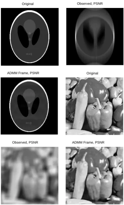
Figure 2. LADMM algorithm for deblurring.

(LADMM) to solve the problem of rapid convergence of the dictionary model that is easy to fall into the local optimal solution. This model combines the

ad-Original Observed, PSNR

ADMM TV, PSNR FTVd, PSNR

Original Observed, PSNR

ADMM Frame, PSNR Original

Observed, PSNR ADMM Frame, PSNR

[image:8.595.272.474.329.664.2]

(9)

vantages of linearization features to make sub-problems easier to solve. When the algorithm is applied to the problem of image reconstruction, we use the quadrat-ic term of the linearized sub-problem to make the sub-problem easier to solve.

Moreover, in the case of similar PSNR, the algorithm does not need regulari-zation operator.

In addition, we analyze the convergence of the LADMM algorithm. Our next step is to generalize the model to more non-convex problems (non-negative ma-trix factorization problems) and use practical problems.

Conflicts of Interest

The author declares no conflicts of interest regarding the publication of this pa-per.

References

[1] Boyd, S., Parikh, N., Chu, E., Peleato, B. and Eckstein, J. (2010) Distributed Opti-mization and Statistical Learning via the Alternating Direction Method of Multip-liers. Foundations and Trends® in Machine Learning, 3, 1-122.

https://doi.org/10.1561/2200000016

[2] Nadai E. (2011) Statistics for High-Dimensional Data: Methods, Theory and Appli-catios. Springer, Berlin.

[3] Wu, Z.M. (2016) Linearized Alternating Direction Method for Solving Separable Convex Optimization Problems.

https://wenku.baidu.com/view/7aff15227ed5360cba1aa8114431b90d6c8589e3.html [4] Fu, X.L., He, B.H., Wang, X.F., et al. (2014) Block-Wise Alternating Direction

Me-thod of Multipliers with Gaussian Back Substitution for Multiple-Block Convex Programming. 1-37.

http://xueshu.baidu.com/usercenter/paper/show?paperid=4cb7be88f0f61a58569089 6f1da8bf31&site=xueshu_se

[5] Wang, H.F. and Kong, L.C. (2017) The Linearized Alternating Direction Method of Multipliers for Sparse Group LAD Model. Beijing Jiaotong University, Beijing. [6] Eckstein, J. (2016) Approximate ADMM Algorithms Derived from Lagrangian

Splitting. Computational Optimization and Applications,68, 363-405.

https://doi.org/10.1007/s10589-017-9911-z

[7] Haubruge, S., Nguyen, V.H. and Strodiot, J.J. (1998) Convergence Analysis and Ap-plications of the Glowinski—Le Tallec Splitting Method for Finding a Zero of the Sum of Two Maximal Monotone Operators. Journal of Optimization Theory and Applications, 97, 645-673.

[8] Glowinski, R. and Marroco, A. (1975) Sur l’approximation, par éléments finis d’ordre un, et la résolution, par Pénalisation-Dualité d’une classe de problèmes de Dirichlet non linéaires. Journal of Equine Veterinary Science, 2, 41-76.

[9] Wang, H.F. (2017) Linearized Multiplier Alternating Direction Method for Solving Least Degree Model of Sparse Group.

https://wenku.baidu.com/view/f25e8ff1d5d8d15abe23482fb4daa58da0111c9c.html [10] Jiao, Y.L., Jin, Q.N., Lu, X.L., et al. (2016) Alternating Direction Method of Multip-liers for Linear Inverse Problems. SIAM Journal on Numerical Analysis, 54, 2114-2137.https://doi.org/10.1137/15M1029308

(10)

[11] Wang, Y.L., Yang, J.F., Yin, W.T., et al. (2016) A New Alternating Minimization Algorithm for Total Variation Image Reconstruction. SIAM Journal on Imaging Sciences, 1, 248–272.