ADAPTIVE DIGITAL PREDISTORTION LINEARISATION
FOR RF POWER AMPLIFIERS
D. Giesbers
1, S. Mann
2, K. Eccleston
11University of Canterbury, Deptartment of Electrical and Computer Engineering.
2
Tait Electronics Ltd, Christchurch Campus. Email: [email protected]
Abstract
Development of linear modulation schemes has opened the way for spectrally efficient, high speed digital communication systems for voice and data applications. A trend has been to develop utra wide and wide bandwidth modulation formats, which has meant feedback linearisation schemes (both analogue and digital) are no longer effective. This has in turn lead to a number of approaches that involve predistorting the signal prior to amplification, with a characteristic that is the inverse to that of the power amplifier (PA). This paper presents a polynomial based predistortion for linearisation of an RF PA. The predistortion characteristic is adaptive, using the LMS algorithm to minimise the mean squared error between output of the PA, and a scaled version of the baseband signal. The simulation of this system indicate that this system can provide 40 dB decrease in ACPR by reducing the 3rd and 5th order IMD products.
Keywords
: digital communications, linearisation, predistortion, RF power amplifier1
Introduction
Recently proposed communication modulation for-mats have opened the way for high-data-rate wire-less communication. In the implementation of dig-ital radio, the effects of non-linearities can be ob-served in a multitude of forms. For example, mix-ers rely on non-linear behaviour to perform their function whereas non-linear behaviour exhibited by power amplifiers can restrict the performance of a system, causing in-band interference and out-of-band noise.
Generation of frequency components not present in the excitation is one effect a non-linear device can exhibit [1]. Of concern in communication sys-tems is the amplitude and phase distortion which causes the signal spectrum to spread, interfering with other bands [2]. Power amplifiers (PAs) can be linearised somewhat by operating in the
lin-ear region. However, to increase output power
levels and efficiency, they are often driven nearer the saturation region. Methods for reducing un-wanted non-linear effects of PAs (while maintain-ing power efficiency) can be broken into three main categories: feedback [3], feedforward [4], and pre-distortion [5].
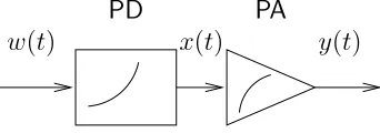
Predistortion linearisation, as depicted in Figure 1, can be used to linearise over a wide bandwidth. This is achieved by predistortion (PD) of the signal prior to amplification with the inverse
characteris-tics of the distortion that will be imposed by the power amplifier. Thus, the output of the PA is a linear function of the input to the predistorter:
y(t) =f(x(t)) (1)
y(t) =f[g(w(t))] =k·w(t) (2)
This paper presents the design and simulation of an adaptive polynomial predistortion linearisation scheme, designed with an end goal of implementa-tion.
PD
PA
y
(
t
)
[image:1.595.330.501.563.623.2]w
(
t
)
x
(
t
)
Figure 1: Basic system diagram of predistortion linearisation
2
Proposed system
The proposed system is depicted in Figure 2. The input to the system will be a quadrature amplitude modulation (QAM) signal, but any baseband modulated signal can be used. Initially, the baseband signal will have a bandwidth of 150kHz. This baseband signal is distorted through a polynomial predistorter before being digitally modulated converted, to an analogue signal, and
amplified. The baseband signal is converted
into polar co-ordinates to allow predistortion of the AM-AM and AM-PM characteristics
independently. The digital modulation and
cartesian to polar conversion can be performed
by a co-ordinate rotation digital computer
(CORDIC) algorithm which can perform a number of trigonometric functions efficiently,
and at high data rates [10]. The output of
the PA is sampled using an analogue to digital converter (ADC), and used in conjunction with the predistorter input to update the predistortion
algorithm. The least means squared (LMS)
algorithm will be used to adjust the polynomial coefficients
DAC RF PA
130 MHz
ADC QAM
Phase Amplitude
Error Coefficient
Subsampling ADC 150 kHz
High Z input
Attenuator divider signal
baseband bandwidth
calculation adjustment
Digital 5th order predisorter
modulator FPGA
polynomial polynomial
or power Coupler
Figure 2: Diagram of the proposed system implementation
3
Amplifier modelling
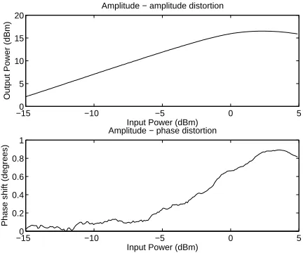
In order to simulate a digital predistortion scheme, a model of a typical PA must first be obtained. For the purposes of this research, a ZFL-2000 amplifier available from Mini Circuits was chosen. The transfer characteristic of this amplifier was measured by performing a power sweep with a HP8753D network analyser. The HP8753D was configured to perform a power sweep at 130 MHz, measuring the amplitude and phase response of the ZFL-2000 amplifier as shown in Figure 3. PA models were developed by fitting a 5th order power series to the collected data using least squares fitting techniques.
Initial verification of the model transfer character-istics were made by comparing two tone test results of the polynomial models with data obtained from a two tone test of the ZFL-2000. The tests were
−150 −10 −5 0 5
5 10 15 20
Input Power (dBm) Amplitude − amplitude distortion
Output Power (dBm)
−150 −10 −5 0 5
0.2 0.4 0.6 0.8 1
Amplitude − phase distortion
Input Power (dBm)
[image:2.595.309.525.74.254.2]Phase shift (degrees)
Figure 3: Measured Transfer characteristic of the ZFL-2000 amplifier
[image:2.595.74.285.375.487.2]carried out at 130 MHz with a tone separation of 150 kHz to correspond to the target operat-ing frequency and bandwidth of the implemented system. The combined input power level of the two tones was varied between -16 dBm and 0dbBm at intervals of 2 dB as the PA, and the extracted models were designed for this range of input power. Figure 4 shows the IMD levels of the PA and PA model. Note that the 5th order model produces the 3rd and 5th order IMD products accurately. This model cannot, however, predict the 7th and higher order IMD products. This is part of the limitations of using a 5th order polynomial model, however raising the order of the model increases the effect of quantisation effect on each IMD product lead-ing to inaccurate modelllead-ing of all IMD products. For this reason a 5th order polynomial PA model was chosen. From Figure 4 we can see that these models are acurate for simulation of the ZFL-2000. The deviation at lower power levels is caused by the noise floor of measurement equipment.
4
Simulation
The LMS algorithm was used to minimise an error function by adapting the power series as described:
An,k+1=Ak+2µekx n
k (3)
Where n = coefficient order, at time = k,Ais the
coefficient vector, x is the input to the adaptive
system,µcontrols convergence and stability of the system, andeis the error calculated as follows:
ek=dk−yk (4)
Wheredk is the desired (undistorted) output from
the system, and yk is the current output of the
−16 −14 −12 −10 −8 −6 −4 −2 0 −120
−100 −80 −60 −40 −20 0
Input (dB)
IMD level (dB)
IMD level, input = 16dBm − 0dBm
[image:3.595.75.289.73.247.2]Meas 3rd Meas 5th Sim 3rd Sim 5th
Figure 4: Two tone test comparison between the ZFL-2000 and power series model, with a input power range of -16 - 0 dBm.
y
kAdapt
x
kG
0 [image:3.595.306.526.90.284.2]d
kFigure 5: LMS diagram adaptive predistortion system
The incoming baseband signal xk is predistorted
with an amplitude expansion, to correct for the compression characteristic of the PA. The base-band signal is also scaled by the gain of the
am-plifier, to form a desired signal dk. The output
from the predistorter is distorted with the transfer characteristic of the PA by a power series to yeild
[image:3.595.76.286.297.392.2]yk. The error is calculated using dk andyk. This error is then used to adjust the coefficients of the predistorter, as detailed above. The only ‘knowl-edge’ of the PA characteristics the system has, is the distorted output that is fed back and used for error calculation and adaption of the coefficients. To simplify the problem for initial investigation of adaptive predistortion, amplitude predistortion was investigated without the added complication of phase distortion.
Figure 6 shows the convergence of the coefficients
of the polynomial power series adaptive
predistorter. The transfer functions of both
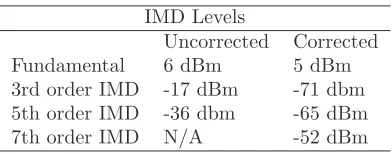
the amplifier and the predistorter are essentially the same as the amplidute transfer functions in Figure 9, and both the corrected and uncorrected spectrum are shown in Figure 7. IMD levels are shown in Table 1.
The above examples of adaptive predistortion deal only with amplitude distortion, however, the PA
0 50 −0.5
0 0.5 1
a
0
0 50 −0.5
0 0.5 1
a
1
Coefficients (y = Σ an xn)
0 50 −0.5
0 0.5 1
a
2
0 50 −0.5
0 0.5 1
a
3
0 50 −0.5
0 0.5 1
a4
0 50 −0.5
0 0.5 1
a5
0 50 −0.5
0 0.5 1
a6
0 50 −0.5
0 0.5 1
a7
Figure 6: Convergence of the coefficients of an amplitude correcting adaptive predistortion linearisation system.
−800 −600 −400 −200 0 200 400 600 800 −140
−120 −100 −80 −60 −40 −20 0 20
Corrected and uncorrected spectrum
Frequency + 130 Mhz (Khz)
Output level (dBm)
Uncorrected Corrected
Figure 7: Corrected and uncorrected spectrum with amplitude predistortion.
IMD Levels
Uncorrected Corrected
Fundamental 6 dBm 5 dBm
3rd order IMD -17 dBm -71 dbm
5th order IMD -36 dbm -65 dBm
7th order IMD N/A -52 dBm
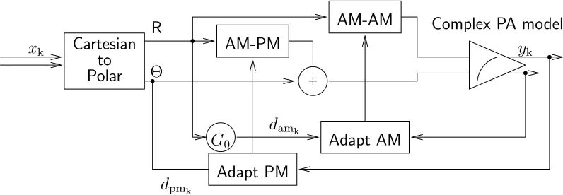
[image:3.595.310.523.375.547.2] [image:3.595.319.515.624.701.2]Θ
R
Cartesian
to
Polar
AM-AM
Adapt AM
d
pmkAdapt PM
x
kComplex PA model
y
kAM-PM
G
0 [image:4.595.94.492.72.210.2]d
amkFigure 8: System diagram of an adaptive predistortion linearisation simulation to correct for both amplitude and phase distortion.
transfer characteristics will introduce both ampli-tude to ampliampli-tude (AM-AM) distortion, and am-plitude to phase (AM-PM) distortion to the ap-plied signal. Thus the predistorter must have fa-cility to apply both an amplitude and phase correc-tive distortion. To simplify the implementation of this, the system has been designed around a polar representation of the signal, and independent AM-AM and AM-AM-PM predistortion power series mod-els. Figure 8 shows how the amplitude and phase predistortion is applied to the baseband inputxk. This system is very similar to the previous ampli-tude only system. The baseband signal is reduced to its magnitude and phase components, to allow for the amplitude and phase predistortion to be applied independently. The transfer functions after the system has had time to converge are shown in Figures 9, which lead to a reduction in the IMD products as shown in Figure 10. IMD levels are shown in Table 2.
−16 −14 −12 −10 −8 −6 −4 −2 0
−20 −10 0 10 20
PA matching LMS polynomial, µ = 0.001 : At 1000000 samples
Input power level (dBm)
Output power level (dBm)
−16 −14 −12 −10 −8 −6 −4 −2 0
−1 −0.5 0 0.5 1
Input power level (dBm)
Phase distortion (degrees)
PA and PD transfer functions PA Polynomial
[image:4.595.75.289.532.716.2]LMS PD Polynomial
Figure 9: Transfer function of the PA and PD providing AM-PM correction
−600 −400 −200 0 200 400 600
−120 −100 −80 −60 −40 −20 0 20
Corrected and uncorrected spectrum
Frequency + 130 Mhz (Khz)
Output level (dBm)
Corrected Uncorrected
Figure 10: Corrected and uncorrected spectrum with amplitude and phase predistortion.
IMD Levels
Uncorrected Corrected
Fundamental 6 dBm 4 dBm
3rd order IMD -18 dBm -85 dbm
5th order IMD -39 dbm -76 dBm
7th order IMD N/A -60 dBm
[image:4.595.319.514.602.679.2]5
Performance
Digital adaptive predistortion implemented using lookup table (LUT) methods have been shown to reduce the 3rd order IMD by between 30 and 40 dB [11] [12]. As can be seen in Figures 7 and 10, 7th order digital adaptive polynomial predisortion can reduce the 3rd order IMD by up to 50 dB and the 5th order IMD by 35 dB. The 7th order predistortion creates 7th order IMD products that increase the total 7th order IMD level by 10 dB, which could be reduced by increasing the order of the predistorter. It should be noted however, that the simulations do not fully show the effects of quantisation. The main restriction of the hard-ware that will be used to implement the proposed system is a 10 bit ADC used to sub sample the RF signal. The effects of this have been simulated by way of 10 bit quantisation between the PA model and the error calculation, with minimal effects to performance. Data paths internal to the FPGA can be as wide as required, so quantisation within the FPGA should not be significant.
Typical LUT implementations have been seen to converge to a new amplifier, or after a channel switch over a time of around 10 seconds although some implementations have improved reduced this [11]. Simulations indicate that convergence to the inverse characteristics of the PA occurs over approximately 70,000 samples. For a system designed around a symbol rate of 150 k/samples, this corresponds to convergence within 0.5 seconds (3rd and 5th IMD products are corrected to below the 7th order IMD level).
6
Conclusion
Digital adaptive polynomial predisortion has a number of benefits over LUT based digital
predistortion approaches. To provide fine
resolution, LUT sizes become very large, which
both increases memory requirements, and
increases adaption time. Polynomial approaches, such as described in this paper, take advantage of current digital signal processing hardware to predistort the signal using a power series. This has significantly smaller memory requirements (only the coefficients for the power series and the current error must be stored) which means that the adaption time is quicker. Simulations indicate that polynomial based predistortion can provide around 40 dB decrease in ACPR, compared with 30 - 40 dB provided by a LUT based approach
References
[1] S. A. Maas, Nonlinear Microwave Circuits.
Artech House, 1988.
[2] M. Faulkner and M. Johansson, “Adaptive linearization using predistortion -
experimen-tal results,”IEEE Transactions on Vehicular
technology, vol. 43, pp. 323–332, May 1994.
[3] S. I. Mann, M. A. Beach, and K. A. Morris, “Digital baseband cartesian loop transmit-ter,” Electronics Letters, vol. 37, pp. 1360– 1361, October 2001.
[4] R. D. Stewart and F. F. Tusubira, “Feed-forward linearisation of 950 mhz amplifiers,” Microwave, Antennas and Propogation IEE proceedings, vol. 135, pp. 347–350, October 1988.
[5] Y. Nagata, “Linear amplification technique
for digital mobile communications,” 1989
IEEE Vehicular Technology Conference (VTC 1989), pp. 159–164, May 1989.
[6] M. Jin, S. K. Shin, D. Oh, and J. Kim, “Re-duced order RLS polynomial predistortion,” Proceedings of the International Symposiam on Circuits and Systems ISCAS, vol. 4, pp. 333 – 336, May 2003.
[7] H. Chen, C. Maa, Y. Wang, and J. Chen, “Joint polymonial and look-up-table power
amplifier linearization scheme,” 2003 IEEE
Vehicular Technology Conference (VTC 2003), vol. 2, pp. 1345–1349, April 2003.
[8] A. Lohtia, P. A. Goud, and C. G. Eng-field, “Power amplifier linearization usin cubic
spline interpolation,” 1993 IEEE Vehicular
Technology Conference (VTC 1993), pp. 676– 679, May 1993.
[9] M. Jin, S. Kim, and D. Oh, “A novel
pre-distorter for power amplifier,” 3rd
Interna-tional conference on Microwave and Millime-ter Wave Technology Proceedings, pp. 1129– 1133, 2002.
[10] R. Andraka, “A survey of CORDIC
algo-rithms for FPGA based computers,”
Proceed-ings of the 1998 ACM/SIGDA Sixth Inter-national Symposium on Field Programmable Gate Arrays, pp. 191–200, March 1998.
[11] J. K. Cavers, “Amplifier linearization using a digital predistorter with fast adaption and low
memory requirements,” 1990 IEEE
Trans-actions on Vehicular Technology, vol. 39, pp. 374–382, November 1990.