Solution of Transportation Problem with South East Corner Method, North East Corner Method and Comparison with Existing Method

(1)

ISSN Print: 2333-9705

DOI: 10.4236/oalib.1105377 Apr. 30, 2019 1 Open Access Library Journal

Solution of Transportation Problem with

South-East Corner Method, North-East Corner

Method and Comparison with Existing Method

Sasikala

1

, Sridhar Akiri

2

, Pavankumar Subbara

3

1_{Department of Mathematics, GIT, GITAM Deemed to Be University, Bangalore Campus, Karnataka, India} 2_{Department of Mathematics, GIT, GITAM Deemed to Be University, Visakhapatnam, Andhra Pradesh, India} 3_{Department of Humanities & Basic Sciences, SBIT Engineering College, Khammam, Telangana, India}

Abstract

Finding an initial basic feasible solution is the prime requirement to obtain an optimal solution for the transportation problems. In this paper, two methods are proposed to find an initial basic feasible solution for the transportation problems. The South-East Corner Method (SECM) and the North-East Cor-ner Method (NECM) are adopted to compute the Initial Basic Feasible Solu-tion (IBFS) of the transportaSolu-tion problem. A comparative study is carried out with existing methods like Vogel’s approximation method (VAM) which is to find an initial basic feasible solution and Modified Distribution (MODI) Me-thod which is to find the optimal solution and the meMe-thods are also illustrated with numerical examples.

Subject Areas

Operational Research

Keywords

Transportation Problem, Initial Basic Feasible Solution (IBFS), Optimal Solution, Transportation Cost, South-East Corner Method (SECM), North-East Corner Method (NECM), Vogel’s Approximation Method (VAM), Modified Distribution Method (MODI)

1. Introduction

Transportation problem is famous in operation research for its wide application in real life. The transportation problem is one of the sub-classes of linear pro-gramming problems. The objective of Transportation Problem is to transport How to cite this paper: Sasikala, Akiri, S. and

Subbara, P. (2019) Solution of Transportation Problem with South-East Corner Method, North-East Corner Method and Comparison with Existing Method. Open Access Library Journal, 6: e5377.

https://doi.org/10.4236/oalib.1105377

Received: April 8, 2019 Accepted: April 27, 2019 Published: April 30, 2019

This work is licensed under the Creative Commons Attribution International License (CC BY 4.0).

http://creativecommons.org/licenses/by/4.0/

(2)

DOI: 10.4236/oalib.1105377 2 Open Access Library Journal various amounts of a single homogeneous commodity that are initially stored in various origins and from there to different destinations in such a way that the total transportation cost is a minimum. The transportation problem received this name because many of its applications involved in determining how to op-timally transport goods. Transportation problem is a logistical problem for or-ganizations especially for manufacturing and transport companies.

The basic transportation problem was originally developed by Hitchcock in 1941 [1]. Efficient methods for finding solution were developed, primarily by Dantzig in 1951 [2] and then by Charnes, Cooper and Henderson in 1953 [3]. Basically, the solution procedure for the transportation problem consists of the following phases:

Phase 1: Mathematical formulation of the transportation problem. Phase 2: Finding an initial basic feasible solution.

Phase 3: Optimizing the initial basic feasible solution which is obtained in Phase 2.

In this paper, Phase 2 has been focused in order to obtain a better initial basic feasible solution for the transportation problems. Again, some of the well re-puted methods for finding an initial basic feasible solution of transportation problems developed and discussed by them are North West Corner Method (NWCM) [4], Least Cost Method (LCM) [4], Vogel’s Approximation Method (VAM) [4] [5], Balakrishnan [6] etc. Then in the next and last stage MODI (Modified Distribution) method was adopted to get an optimal solution. Charnes and Cooper [3] also developed a method for finding an optimal solution from IBFS named as “Stepping Stone Method”.

Recently, R. A. Lakshmi and P. L. Pallavi [7], Vinoba and Palaniyappa [8], Al-fred Asase [9], Francois Ndayiragije [10] proposed different methods to obtain initial basic feasible solutions.

In this paper, we introduce the South East Corner Method and North East Corner Methods used to obtain an initial basic feasible solution for the trans-portation problems. A comparative study is also carried out by solving a good number of transportation problems which show that the proposed methods give better result in comparison to the other existing methods available in the litera-ture.

2. Network Representation and Mathematical Formulation

of the Transportation Problem

(3)

[image:3.595.218.527.70.225.2]

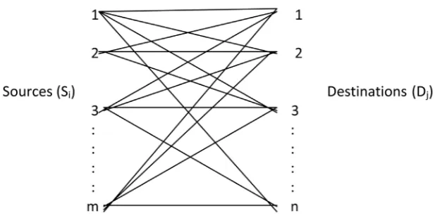
DOI: 10.4236/oalib.1105377 3 Open Access Library Journal Figure 1. Network representation of transportation problem.

In developing the Linear Programming model of a transportation problem the following notations are used

Transportation problem

1 1 Min m n ij ij

i j

Z C X

= =

=

∑∑

Subject to

1 , 1,2, , n

ij i

j

x S i m

=

≤ =

∑



1 , 1,2, , m

ij j

i= x D j n

≥ =

∑



and xij ≥ 0, for all i and j.

The objective function minimizes the total cost of transportation Z between various sources and destinations. The constraint i in the first set of constraints ensures that the total units transported from the source I is less than or equal to its supply. The constraint j in the second set of constraints ensures that the total units transported to the destination j is greater than or equal to its demand.

Feasible solution: A set of non negative values xij, i = 1, 2, …, n and j = 1, 2, …, m that satisfies the constraints is called a feasible solution to the transpor-tation problem.

Optimal solution: A feasible solution is said to be optimal if it minimizes the total transportation cost.

Non degenerate basic feasible solution: A basic feasible solution to a (m × n) transportation problem that contains exactly m + n – 1 allocations in inde-pendent positions.

3. Proposed Methods to Obtain Initial Basic Feasible

Solution

3.1. South East Corner Method

The steps involved in solving the transportation problem using south east corner method is given below.

(4)

DOI: 10.4236/oalib.1105377 4 Open Access Library Journal problem is balanced.

Step 2: The method starts at the south east corner cell of the table (variable (xmn).

Step 3: Allocate as much as possible to the selected cell and adjust the asso-ciated amounts of supply and demand by subtracting the allocated amount.

Step 4: Cross out the row or column with zero supply or demand to indicate that no further assignments can be made in that row or column. If both a row and column net to zero simultaneously, cross out one only and leave a zero supply (demand in the uncrossed out row-column).

Step 5: If exactly one row or column is left uncrossed out, stop. Otherwise, move to the cell to the right if a column has just been crossed out. Go to step 3.

3.2. North East Corner Method Procedure

The steps involved in solving the transportation problem using north east corner method are given below.

Step 1: The method starts at the North east corner cell of the tableau (variable X1n).

Step 2: Allocate as much as possible to the selected cell and adjust the asso-ciated amounts of supply and demand by subtracting the allocated amount.

Step 3: Cross out the row or column with zero demand to indicate that no further assignments can be made in the row or column. If both row and column net to zero simultaneously cross out one only and leave a zero supply (demand in the uncrossed out row or column).

Step 4: If exactly one row or column is left uncrossed out or below if exactly one row or column is left uncrossed out, stop. Otherwise, move to the cell to the right if a column has just been crossed out or below if a row has been crossed out. Go to step 1.

Step 5: Start with X1n and end at Xm1.

3.3. Vogel’s Approximation Method (VAM)

The Vogel approximation method is an iterative procedure for computing a ba-sic feasible solution of the transportation problem.

Step 1: Identify the boxes having minimum and next to minimum transportion cost in each row and write the difference (penalty) along the side of the ta-ble against the corresponding row.

Step 2: Identify the boxes having minimum and next to minimum transporta-tion cost in each column and write the difference (penalty) against the corres-ponding column.

Step 3: Identify the maximum penalty. If it is along the side of the table, make maximum allotment to the box having minimum cost of transportation in that row. If it is below the table, make maximum allotment to the box having mini-mum cost of transportation in that column.

(5)

DOI: 10.4236/oalib.1105377 5 Open Access Library Journal Step 5: Continue the procedure until the total available quantity if fully allo-cated to the cells as required.

3.4. Test for Optimality

Once an initial solution is obtained, the next step is to check its optimality. An optimal solution is one where there is no other set of transportation routes (al-locations) that will further reduce the total transportation cost. Thus, we have to evaluate each unoccupied cell (represents unused route) in the transportation table in terms of an opportunity of reducing total transportation cost. An unoc-cupied cell with the largest negative opportunity cost is selected to include in the new set of transportation routes (allocations). This is also known as an incoming variable. The outgoing variable in the current solution is the occupied cell (basic variable) in the unique closed path (loop) whose allocation will become zero first as more units are allocated to the unoccupied cell with largest negative opportu-nity cost. Such an exchange reduces total transportation cost. The process is continued until there is no negative opportunity cost. That is, the current solu-tion cannot be improved further. This is the optimal solusolu-tion. An efficient tech-nique called the modified distribution (MODI) method (also called U-V Me-thod). Now we discuss MODI method which gives optimal solution and is shown in below.

Modified Distribution (MODI) Method

Step 1: Determine an initial basic feasible solution using any one of the methods which are namely, North West Corner Method, Least Cost Method and Vogel’s Approximation Method.

Step 2: Determine the values of dual variables, Ui and Vj using Ui + Vj = Cij. Step 3: Compute the opportunity cost using dij = Cij – (Ui + Vj) from unoccu-pied cell.

Step 4: Check the sign of each opportunity cost (dij). If the opportunity costs of all the unoccupied cells are either positive or zero, the given solution is the optimum solution. On the other hand, if one or more unoccupied cell has nega-tive opportunity cost, the given solution is not an optimum solution and further savings in transportation cost are possible.

Step 5: Select the unoccupied cell with the smallest negative opportunity cost as the cell to be included in the next solution.

Step 6: Draw a closed path or loop for the unoccupied cell selected in the pre-vious step. Please note that the right angle turn in this path is permitted only at occupied cells and the original unoccupied cell.

Step 7: Assign alternate plus and minus signs at the unoccupied cells on the corner points of the closed path with a plus sign at the cell being evaluated.

(6)

DOI: 10.4236/oalib.1105377 6 Open Access Library Journal with plus signs and subtract it from those cells marked with minus signs. In this way an unoccupied cell becomes an occupied cell.

Step 9: Repeat the whole procedure until an optimum solution is obtained.

4. Numerical Examples with Illustration

4.1. Example

A company has three warehouses, W1, W2 and W3, which are supplied by three suppliers, S1, S2 and S3. The table shows the cost Cij of sending one case of goods from supplier Si to warehouse Wj, in appropriate units. Also shown in the table are the number of cases available at each supplier and the number of cases re-quired at each warehouse.

Consider the following balanced transportation problem.

From\To W1 W2 W3 Availability

S1 10 4 11 14

S2 12 5 8 10

S3 9 6 7 6

Requirement 8 10 12

4.1.1. South East Corner Method

By applying South East Corner Method the allocations are obtained as follows:

From\To W1 W2 W3 Availability ai

S1 10 4 11 a1 = 14

S2 12 5 8 a2 = 10

S3 9 6 7 a3 = 6

Requirement bj b1 = 8 b2 = 10 b3 = 12

3 3

1 i 1 j 30

j= a i= b

= =

∑

It is a balanced transportation problem as

1 1 30.

n m

i j

j= a i= b

= =

∑

1) At the beginning we have a matrix of order 3X3, firstly we choose the south east corner cell of the table (x33), i.e., from (3, 3) cell. Here min (S3, W3) = min (6, 12) = 6 units. Therefore the maximum possible units that can be allocated to this cell is 6 and it as 6 (7) in the cell (3, 3). This completes the allocation in the 3rd row and cross the other cells, i.e., (3, 1) and (3, 2) in the row.

S1 14

S2 10

S3 ₍₆₎7 6 − 6 = 0

(7)

DOI: 10.4236/oalib.1105377 7 Open Access Library Journal 2) After completion of step.1 come to cell (2, 3) here min (10, 12 − 6 = 6) = 6 units can be allocated to the cell and write it as 6 (8). This completes the alloca-tion in the 3rd_{column and cross the other cells in that column.}

S1 X 14

S2 ₍₆₎8 10 − 6 = 4

S3 X X ₍₆₎7 0

Requirement bj 8 10 6 − 6 =0 18

3) Now come to second column, here the cell (2, 2) is min (10 − 6 = 4, 10) = 4 units can be allocated to this cell and write it as 4 (5). This completes the alloca-tions in second row so cross the other cells in that row.

S1 X 14

S2 X ₍₄₎5 ₍₆₎8 4 − 4 = 0

S3 X X ₍₆₎7 0

Requirement bj 8 10 − 4 = 6 0 14

4) Again consider the position (1, 2). Here min (14, 10 − 4 = 6) = 6 units can be allocated to this cell and write it as 6 (4). This completes the allocations in second column.

S1 ₍₆₎4 X 14 – 6 = 8

S2 X ₍₄₎5 ₍₆₎8 0

S3 X X ₍₆₎7 0

Requirement bj 8 0 0 8

5) Finally, allocate the remaining units to the cell (1, 1), i.e., 8 units to this cell and write it as 8 (10).

6) All allocations done in the above tables and complete the table as follows:

S1 ₍₈₎10 ₍₆₎4 11 14

(8)

DOI: 10.4236/oalib.1105377 8 Open Access Library Journal Continued

S3 9 6 7 (At first) ₍₆₎ 6

Requirement 8 10 12

From the above table the initial basic feasible solution is given by X11 = 8, X12 = 6, X22 = 4, X23 = 6, X33 = 6.

The total cost associated with these allocations = 10 × 8 + 4 × 6 + 5 × 4 + 8 × 6 + 7 × 6 = 214.

4.1.2. North East Corner Method

By applying North East Corner Method the allocations are obtained as follows:

S1 10 ₍₂₎4 11 (At first) ₍₁₂₎ 14

S2 ₍₂₎12 ₍₈₎5 8 10

S3 ₍₆₎9 6 7 6

Requirement 8 10 12

The initial basic feasible solution is given by X12 = 2, X13 = 12, X21 = 2, X22 = 8, X31 = 6.

4.1.3. Vogel’s Approximation Method (VAM Method) (Existing Method)

To find the initial basic feasible solution for the above example Vogel’s approx-imation method is used and allocations are obtained as follows:

By applying VAM process allocations are obtained as follows:

From\To W1 W2 W3 Availability Penalty (1) Penalty (2) Penalty (3)

S1 ₍₄₎10 ₍₁₀₎4 11 \14 4 6 1 1

S2 12 5 ₍₁₀₎8 \10 3 4 -

S3 ₍₄₎9 6 ₍₂₎7 \6 4 1 2 2

Requirement \8 4 \10 \12 \2 30\30

Penalty (1) 1 1 1

Penalty (2) 1 - 1

Penalty (3) 1 - 1

(9)

DOI: 10.4236/oalib.1105377 9 Open Access Library Journal The total cost associated with these allocations = 10 × 4 + 4 × 10 + 8 × 10 + 9 × 4 + 7 × 2 = 210.

4.1.4. Optimal Solution Using MODI Method

From\To W1 W2 W3 Availability Ui

S1 ₍₄₎10 ₍₁₀₎4 11 8 ₃ 14 U1 = 0

S2 12 10 ₂ 5 4 ₁ ₍₁₀₎8 10 U2 = 0

S3 ₍₄₎9 6 3 ₃ ₍₂₎7 6 U3 = −1

Requirement 8 10 12

Vj V1 = 10 V2 = 4 V3 = 8

Finding Ui and Vjvalues from occupied cells

Here we find Ui and Vjvalues by assuming U1 = 0 then we will find remaining Ui and Vj values.

From the occupied cells (Ui + Vj = Cij). U1 = 0;

U1 + V1 = 10 U1 + V2 = 4 U3 + V1 = 9 U3 + V3 = 7 U2 + V3 = 8. 0 + V1 = 10 0 + V2 = 4 U3 + 10 = 9 −1 + V3 = 7 U2 + 8 = 8. V1 = 10 V2 = 4 U3 = 9 − 10 = −1 V3 =7 + 1 = 8 U2 = 0. U1 = 0; U2 = 0; U3 = −1; V1 = 10; V2 = 4; V3 = 8.

Finding dij = Cij− (Ui + Vj) for unoccupied cells d13 = C13 − (U1 + V3) = 11 − (0 + 8) = 3. d21 = C21 − (U2 + V1) = 12 − (0 + 10) = 2. d22 = C22 − (U2 + V2) = 5 − (0 + 4) = 1. d32 = C32 − (U3 + V2) = 6 − (−1 + 4) = 3.

Here Ui + Vj values of each unoccupied cell are showing in the cell of top right corner value and dij values are in down right corner of each cell. All dij values are positive we get optimal solution.

So, the total cost associated with these allocations = 10 × 4 + 4 × 10 + 8 × 10 + 9 × 4 + 7 × 2 = 210.

To get optimal solution MODI (Modified Distribution) method is adopted and by applying MODI method the optimal solution is obtained as 210.

4.2. Example

Consider the transportation problem given by the following table of supply, de-mand and unit costs.

A B C Supply

1 10 12 9 40

2 4 5 7 50

3 11 8 6 60

(10)

DOI: 10.4236/oalib.1105377 10 Open Access Library Journal

4.2.1. South East Corner Method

By applying south east corner rule process allocations are obtained as follows:

A B C Supply

1 ₍₄₀₎10 40

2 ₍₃₀₎4 ₍₂₀₎5 50

3 ₍₃₀₎8 6 (At First) ₍₃₀₎ 60

Demand 70 50 30

4.2.2. North East Corner Method

By applying North East Corner Method the allocations are obtained as follows:

A B C Supply

1 ₍₁₀₎12 9 (At first) ₍₃₀₎ 40

2 ₍₁₀₎4 ₍₄₀₎5 50

3 ₍₆₀₎11 60

Demand 70 50 30

4.2.3. VAM Method

To find the initial basic feasible solution for the above example Vogel’s approx-imation method is used and allocations are obtained as follows:

A B C Supply

1 ₍₂₀₎10 ₍₂₀₎9 40

2 ₍₅₀₎4 50

3 ₍₅₀₎8 ₍₁₀₎6 60

(11)

DOI: 10.4236/oalib.1105377 11 Open Access Library Journal The total cost associated with these allocations = 10 × 20 + 9 × 20 + 4 × 50 + 8 × 50 + 6 × 10 = 1040.

4.2.4. Optimal Solution Using MODI Method

A B C Supply Ui

1 ₍₂₀₎10 12 11 ₁ ₍₂₀₎9 40 U1 =0

2 ₍₅₀₎4 5 5 ₀ 7 3 ₄ 50 U2 = -6

3 11 7 ₄ ₍₅₀₎8 ₍₁₀₎6 60 U3 = −3

Demand 70 50 30

Vj V1 =10 V2 = 11 V3 = 9

Here all dij’s are positive, we get optimal solution.

5. Result Analysis

Methods Total Transportation Cost

Example 1 Example 2

South-East Corner Method 214 1040

North-East Corner Method 258 1290

Vogel’s Approximation Method 210 1040

MODI Method (optimal solution) 210 1040

It can be shown that the value obtained by South-East Corner Method, North-East Corner Method is near to the optimal solution and also by the North-East Corner Method is not nearer to the optimal solution which obtained by MODI method(optimal solution). Since the South-East Corner Method is better initial solution than the North-East Corner Method.

6. Conclusion

In this paper, we gave the SECM and NECM which are new methods used to obtain initial basic feasible solutions in transportation problem and compared with Vogel’s approximation and Modified Distribution Method (existing) for optimal solution. Thus, it can be concluded that South-East Corner Method provides an optimal solution directly or in fewer iterations and North-East Cor-ner Method gives an optimal solution for more iterations, for the transportation problems. So South-East Corner Method takes less time and easy to apply for the decision makers who are dealing with logistic and supply chain problems.

Conflicts of Interest

(12)

DOI: 10.4236/oalib.1105377 12 Open Access Library Journal

References

[1] Hitchcock, F.L. (1941) The Distribution of a Product from Several Sources to Nu-merous Localities. Journal of Mathematics and Physics, 20, 224-230.

https://doi.org/10.1002/sapm1941201224

[2] Dantzig, G.B. (1951) Application of the Simplex Method to a Transportation Prob-lem, Activity Analysis of Production and Allocation. John Wiley and Sons, New York, 359-373.

[3] Charnes, A., Cooper, W.W. and Henderson, A. (1953) An Introduction to Linear Programming. John Wiley & Sons, New York.

[4] Hamdy, A.T. (2007) Operations Research: An Introduction. 8th_{Edition, Pearson} Prentice Hall, Upper Saddle River.

[5] Pandian, P. and Natarajan, G. (2010) A New Approach for Solving Transportation Problems with Mixed Constraints. Journal of Physical Sciences, 14, 53-61.

[6] Balakrishnan, N. (1990) Modified Vogel’s Approximation Method for Unbalanced Transportation Problem. Applied Mathematics Letters, 3, 9-11.

https://doi.org/10.1016/0893-9659(90)90003-T

[7] Lakshmi, R.A. and Pallavi, P.L. (2015) A New Approach to Study Transportation Problem Using South West Corner Rule. International Journal of Advanced Re-search Foundation, 2, 1-3.

[8] Vinoba, V. and Palaniyappa, R. (2014) A Study on North East Corner Method in Transportation Problem and Using of Object Oriented Programming Model (C++). International Journal of Mathematics Trends and Technology, 16, 1-8.

[9] Asase, A. (2011) The Transportation Problem; Case Study. A Thesis Submitted to the Department of Mathematics Faculty of Physical Science and Technology, Ku-masi, 7 June 2011.