Accelerated Entry Point Search Algorithm for Real-Time Ray-Tracing
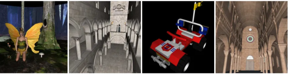
Figure 1: Four of the scenes used for testing purposes. From the left: “Fairy Forest” from the Utah 3D Animation Repository, Legocar from
the Ompf forum model repository and Marko Dabrovic’s Sponza Atrium and Sibenik Cathedral
Abstract
1
Traversing an acceleration data structure, such as the Bounding Vol-2
ume Hierarchy or kD-tree, takes a significant amount of the total 3
time to render a frame in real-time ray tracing. We present a two-4
phase algorithm based upon MLRTA for finding deep entry points 5
in these tree acceleration data structures in order to speed up traver-6
sal. We compare this algorithm to a base MLRTA implementation. 7
Our results indicate an across-the-board decrease in time to find the 8
entry point and an increase in entry point depth. The overall per-9
formance of our real-time ray-tracing system shows an increase in 10
frames per second of up to 36% over packet-tracing and 18% over 11
MLRTA. The improvement is algorithmic and is therefore applica-12
ble to all architectures and implementations. 13
CR Categories: I.3.7 [Three-Dimensional Graphics and
Re-14
alism]: Raytracing, Beam Tracing.— [I.3.6]: Methodology and 15
Techniques—Graphics data structures and data types. 16
Keywords: real-time ray-tracing, MLRTA, BVH, kD-tree,
traver-17
sal algorithm 18
1
Introduction
19
The na¨ıve ray-tracing algorithm involves the tracing of single rays 20
through every object in the scene database to determine the inter-21
section nearest to the ray origin [Appel 1968] [Whitted 1980] [Cook 22
et al. 1984]. Modern ray-tracers use an acceleration data structure, 23
such as the BVH or kD-tree, to reduce the candidate set for intersec-24
tion fromNobjects tologN[Glassner 1989]. Up to 60% of total 25
rendering time is spent traversing these acceleration data structures 26
[Benthin 2006]. The simple tracing of single rays through an ac-27
celeration data structure, such as the kD-tree or Bounding Volume 28
Hierarchy, which we refer to as “mono-tracing”, was first improved 29
upon by traversing multiple rays at once [Havran and Bittner 2000]. 30
Packet-tracing [Wald et al. 2001] [Wald 2004] [Benthin 2006] is 31
a technique that groups coherent rays (that is, rays with relatively 32
similar directional vectors and origin point components) together to 33
trace them through the acceleration data structure simultaneously. 34
Highly coherent ray packets will tend to traverse the tree in the same 35
fashion. By leveraging the SIMD capabilities of modern CPU ar-36
chitectures, several or all the rays in a packet can be operated on at 37
once. 38
2
MLRTA
39
The Multi Level Ray-Tracing Algorithm (MLRTA) [Reshetov et al. 40
2005] further extends the concept of packets to a more general case 41
by using a ray proxy frustum. This frustum is typically composed 42
of the corner rays of a large packet. It acts as a proxy for rays that 43
lie inside the frustum, regardless of whether or not these rays have 44
actually been generated yet. At its simplest, the ray proxy frustum 45
may be used for trivial rejects against the axis-aligned bounding 46
box (AABB) of the scene geometry. We may, for example, form a 47
ray proxy frustum that bounds a set of primary rays corresponding 48
to a tile on the image plane. If the ray proxy frustum does not 49
intersect the AABB, we can conclude that all rays inside the ray 50
proxy frustum do not intersect it either. 51
2.1 Entry Points
52
It is possible that a ray proxy frustum may traverse the tree and end 53
up wholly in a single leaf. For example, when traversing a kD-tree, 54
the ray proxy frustum may not overlap any splitting planes. As the 55
frustum serves as a proxy for any rays in the frustum, logically, any 56
one of these rays traversing the kD-tree will end up in the same 57
single leaf. Therefore, as we know the ray will end up in a specific 58
leaf, there is no need to traverse the tree at all. We may simply 59
intersect the ray with any objects in the leaf. We therefore say that 60
the traversal algorithm enters the tree at that leaf node. The leaf 61
node is our entry point into the tree. 62
The above illustrates an extreme case where the ray proxy frustum 63
does not overlap any split planes and hence no other leaf nodes so 64
that the entry point is at a leaf node, requiring no traversal. In a case 65
where the ray proxy frustum overlaps two leaf nodes containing 66
objects, both children of a common parent, the entry point is the 67
parent node as rays inside the ray proxy frustum may terminate in 68
either node. If one of the leaf nodes contained no objects we may 69
safely ignore it as no intersections will occur in that leaf. The entry 70
point is then the other leaf node. 71
“the common ancestor node in the tree of all leaves that contain
73
objects overlapped fully or partially by the ray proxy frustum”
74
2.2 Entry Point Search
75
MLRTA is implemented using the following procedure: 76
• Prepare a stack data structure capable of holding kD-tree 77
nodes and the corresponding AABB of the node in the 78
kD-tree together in a single stack element. This is termed the 79
bifurcation stack. 80
81
• Starting at the root node, begin traversing the kD-tree with 82
the ray proxy frustum. 83
84
• If the ray proxy frustum must traverse both children of the 85
current node, the current node and current AABB are pushed 86
onto the bifurcation stack. 87
88
• The kD-tree is traversed using the ray proxy frustum until the 89
first occupied leaf is found. 90
91
• The bifurcation stack is now frozen. No further entries may 92
be added to it. The current leaf is marked as the current entry 93
point candidate. 94
95
• For each node on the bifurcation stack, mark the node as 96
a possible candidate and investigate if the tree branch not 97
previously taken below that node contains an occupied leaf 98
overlapped by the ray proxy frustum. If so, the possible 99
candidate is marked as the new entry point. 100
101
• Continue until the bifurcation stack is empty. 102
103
• Return the current entry point as the entry point into the tree 104
for all rays proxied by the frustum. The AABB stored on 105
the bifurcation stack with the entry point is also returned for 106
kD-tree traversal. 107
108
3
Accelerated Entry Point Search Algorithm
109
MLRTA’s entry point search algorithm may be broken down into 110
two phases, namely: 111
1. Traverse the tree with the ray frustum proxy, preparing a 112
candidate list of entry points. 113
114
2. Investigate the candidate list, returning the best1entry point.
115
116
We enhance both of these phases, returning deeper entry points in 117
phase 1 and visiting fewer nodes in phase 2. As the kD-tree acceler-118
ation data structure is a binary tree, finding an entry point one node 119
deeper into the tree reduces the number of nodes under the entry 120
point (assuming a complete binary tree2) by half, therefore in the 121
best case halving the number of nodes visited during the traversal 122
1We define the best entry point as the node which the minimum number of traversal steps are necessary for all in the rays in the proxy frustum to reach a leaf node containing objects.
2A binary tree in which all leaf nodes are at the same depth.
of the acceleration data structure by rays which the frustum prox-123
ies. Deeper entry points are also beneficial on GPUs where stacks 124
are difficult to implement due to hardware constraints [Foley and 125
Sugerman 2005]. As the stack size required for a full traversal from 126
entry point to leaf isdl−de, wheredlis the leaf depth anddethe 127
depth of the entry point, by increasingde, we lower memory re-128
quirements and the possibility that stack restarts are required when 129
using a GPU tree traversal algorithm with a limited stack size [Horn 130
et al. 2007]. 131
By finding the entry point faster, we accelerate the traversal of the 132
kD-tree, yielding more CPU time for triangle intersection and shad-133
ing, ultimately culminating in an increase in renderer throughput. 134
3.1 Phase 1
135
Phase one of our algorithm prepares an entry point candidate list 136
in a similar fashion to MLRTA. We traverse the ray proxy frustum 137
through the kD-tree, adding nodes where both children must be tra-138
versed to the candidate list. As there is a high probability that a ray 139
proxy frustum reaching a leaf node does not actually intersect with 140
any object in that leaf node [Reshetov 2007], we do not freeze the 141
candidate list until the ray proxy frustum has reached a leaf in which 142
it actually overlaps objects stored in the leaf. In contrast, MLRTA 143
stops when it reaches any full leaf node, regardless of whether the 144
ray proxy frustum overlaps objects stored in that leaf or not. 145
Frustum Culling
146
In order to ascertain whether the ray proxy frustum has reached a 147
leaf in which it overlaps an object, we employ a simple plane-based 148
test. If all of an object’s triangles are on the outer side of a plane 149
formed by a frustum face, it is not intersected by the ray proxy frus-150
tum. A dot product is used to test if all of a triangle’s vertices are 151
on the same side of a plane. If the signs of the dot products of each 152
vertex are the same then the triangle does not overlap the plane. 153
Using SIMD, we are able to concurrently test all four planes of the 154
ray proxy frustum. The normals of the frustum planes are already 155
pre-calculated in order to cull kD-tree nodes and thus there is lit-156
tle overhead to this test. This phase is similar to the shaft culling 157
techniques presented in [Dmitriev et al. 2004]. 158
3.2 Phase 2
159
The candidate list contains the nodes on a traversal from root to 160
overlapped leaf where the ray proxy frustum possibly overlaps both 161
child sub-trees of that node. The candidate nodes are therefore or-162
dered by depth. Candidate nodes at lower levels exist in sub-trees of 163
higher nodes. Therefore, if we can ascertain that both of a candidate 164
entry point’s sub-trees contain leaves overlapped by the ray proxy 165
frustum, we know that any entry point below the current entry point 166
will not encompass all of the sub-trees of the current candidate. We 167
can therefore cull all entry points in a candidate list at a tree depth 168
below any point found with both sub-trees containing leaves with 169
overlapped objects . 170
As investigating each potential entry point involves a traversal from 171
that point to an occupied leaf, by not having to test every entry 172
point we greatly decrease the nodes traversed and therefore the time 173
required to perform such traversals. As the Accelerated Entry Point 174
Search Algorithm (AEPSA) performs tests in a top-down manner 175
from the highest potential entry point, when it is known that an 176
entry point cannot be deeper in the tree than the current point, we 177
may reject any nodes remaining in the list. MLRTA performs a 178
bottom-up test of entry point candidates and therefore requires each 179
The candidate list/bifurcation stack is populated by a root to leaf 181
traversal of a tree withnnodes, therefore it will contain at least 182
one node (the leaf the traversal terminates in) and at most logn
183
nodes (each node visited in the traversal, if the ray proxy frustum 184
overlaps both child nodes). The number of possible entry points 185
in the list/stack can therefore be written asp(logn)where p is a 186
“branching factor” and0< p≤1. 187
During phase 2, in a candidate list/stack withkentries, MLRTA will 188
visitk(logn)nodes. This is because each entry in the stack requires 189
a traversal from that candidate entry point to a leaf. AEPSA will 190
visitx(logn), wherex≤kas AEPSA can exit early as soon as it 191
encounters a candidate with a child with an overlapped, occupied 192
leaf. The bounds ofxare1≤x≤logn. We can therefore prove 193
that AEPSA will at worst spend the same time as MLRTA searching 194
for the entry point and at no point will it spend longer. 195
By using this entry point test procedure, we yield the same entry 196
points as MLRTA when considering the same candidate list but 197
without requiring the entire candidate list search. 198
3.3 Algorithm Outline
199
AEPSA is implemented using the following procedure: 200
• Prepare a queue data structure capable of holding AABBs 201
and tree nodes together in a single stack element. This is 202
termed the entry point candidate queue. 203
204
• Starting at the root node, begin traversing the kD-tree with 205
the ray proxy frustum. 206
207
• If the ray frustum must traverse both children of the current 208
node, the current node and current AABB are added to the 209
entry point candidate queue. 210
211
• The kD-tree is traversed using the ray proxy frustum until the 212
first occupied leaf is found that contains objects intersected 213
by the ray proxy frustum 214
215
• The entry point candidate queue is now frozen. No further 216
entries may be added to it. 217
218
• Take the first candidate from the queue and set it as the 219
candidate entry point. Investigate if the kD-tree branch not 220
previously taken below that candidate entry point node con-221
tains an occupied leaf overlapped by the ray proxy frustum. 222
If so, return the current entry point. The AABB stored with 223
the entry point is also returned for kD-tree traversal. 224
225
• If necessary, continue until the queue is empty. 226
227
Figure 2 illustrates the full algorithm and compares it with a ML-228
RTA entry point search into the same kD-tree. A traversal by ML-229
RTA from root to the first occupied leaf in this instance will yield 230
the bifurcation stack [2,1,0] (Node 2 being at the top of the stack 231
and 0 at the bottom). After testing node 2, 1 and 0, MLRTA will 232
return 0 as the entry point into the tree as an occupied leaf 9 is also 233
overlapped by the ray proxy frustum. AEPSA on its search for the 234
first occupied leaf containing triangles overlapping the ray proxy 235
frustum will yield the candidate queue [9]. As this is the only can-236
didate in the queue, we return 9 as the entry point. AEPSA in this 237
case has produced an entry point 3 levels deeper into the tree and 238
instead of entering all rays proxied by the frustum at the root, en-239
ters them at a leaf node meaning that no traversal is required. See 240
Appendix A for a pseudo-code implementation of AEPSA. 241
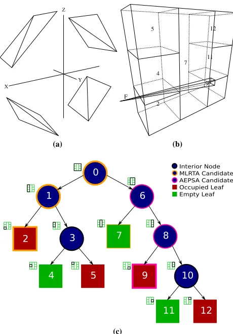
Z
Y X
(a)
5 12
7
9
2 4
F
11
(b)
(c)
Figure 2: (a) A simple scene formed by eight triangles inclined at
a45◦angle to the XY plane. (b) A visualisation of the leaf nodes
formed by a kD-tree compiler using a termination criterion of a maximum of 2 triangles per leaf. Also shown is an example ray proxy frustum that enters the scene from the left, penetrating leaf node 2, but missing the triangles in the leaf. The ray proxy frustum continues on, finally penetrating two triangles in leaf node 9. (c) A layout of the kD-tree compiled in (b).
4
Comparison with MLRTA
242
We begin our comparisons of AEPSA to MLRTA by considering 243
two extreme cases. We compare the number of nodes visited by 244
both. 245
Case one (see Figure 3) consists of a complete balanced kD-tree 246
containingN nodes in which all leaf nodes contain objects. The 247
ray proxy frustum fully overlaps the entire tree and therefore every 248
object in all leaves. The common ancestor of all intersected occu-249
pied leaves is then the root node. The traversal from root to the first 250
occupied leaf addslogN candidates to the bifurcation stack and 251
in the case of AEPSA, the entry point candidate queue. To check 252
each candidate entry point, a traversal of the tree from the candi-253
date node to a leaf is performed. Each traversal will visitlogN
254
nodes. As MLRTA will perform a traversal for each node on the bi-255
furcation stack, the number of visited nodes isN. Given that each 256
leaf is fully overlapped by the ray proxy frustum, during phase 2 257
[image:3.595.321.551.94.423.2](a)
[image:4.595.60.288.55.265.2](b)
Figure 3: A comparison of the visited nodes in a tree where the ray
proxy frustum fully overlaps each leaf. (a) MLRTA: a traversal from the root node 0 to the first occupied leaf 3 adds the nodes [3,1,0] to the bifurcation stack. 3 is popped and marked as a potential entry point. Node 1 is then popped and investigated. As a traversal from 1 to 4 finds an occupied leaf, the candidate entry point is now 1. Node 0 is then popped. A traversal from node 0 passes through node 2 to an occupied leaf at 5. Node 0 is then marked as the candidate entry point. As the stack is now empty the current entry point 0 is returned. (b) AESPA: a traversal from the root node 0 to the first occupied overlapped leaf 3 adds the nodes [0,1,3] to the candidate queue. The first entry (and highest in the tree) 0 is investigated and a traversal from 0 to leaf 5 yields an occupied overlapped leaf. Node 0 is returned as the entry point.
candidate (the tree root node) in the candidate queue. At this point, 259
AEPSA will return the root node as the entry point after a single 260
logNtraversal. 261
Case two (see Figure 4) consists of a complete balanced kD-tree 262
containingN nodes, in which 50% of all leaf nodes contain ob-263
jects. The ray proxy frustum overlaps two empty leaf nodes and a 264
single occupied leaf node. The common ancestor of all intersected 265
occupied leaves is therefore the leaf node itself. MLRTA performs 266
a traversal from the root node 0 to the first occupied leaf 3 and adds 267
the nodes [3,1,0] to the bifurcation stack. Node 3 is popped and 268
marked as a potential entry point. Node 1 is then popped and inves-269
tigated. As a traversal from 1 to 3 finds an empty leaf, the candidate 270
entry point is still leaf 3. Node 0 is then popped and investigated. 271
A traversal from the candidate 0 along the right sub-tree visits in 272
order, the nodes 2, 5 and 6. As leaf 5 is empty and leaf 6 is not 273
overlapped, the candidate entry point is still leaf node 3. The bifur-274
cation node is now empty, therefore node 3 is returned as the entry 275
point. AEPSA performs a traversal from the root node 0 to the first 276
occupied overlapped leaf 3 and adds the nodes [0,1,3] to the candi-277
date queue. The first entry (and highest in the tree) 0 is investigated 278
and traverses in order, the nodes 2, 5 and 6. As there is no overlap, 279
AEPSA has not yet found an entry point. Node 1 is then taken from 280
the queue. As node 4 is empty, AEPSA has not yet found the entry 281
point. The final node 3 is taken from the queue. As it is the last 282
entry in the queue and is occupied, it is by definition overlapped by 283
the ray proxy frustum and is returned as the entry point 284
Figure 4: A comparison of the visited nodes in a tree where the
ray proxy frustum fully overlaps leaves 3, 4 and 5. Leaf 6 is not overlapped by the ray proxy frustum.
The traversal from root to the first occupied leaf (also the only over-285
lapped leaf) addslogNcandidates to the bifurcation stack or, in the 286
case of AEPSA, the entry point candidate queue. MLRTA will mark 287
the leaf as a potential entry point and test all the leaves above it in 288
the leaf again yieldinglogNlogNnodes visited. As AEPSA starts 289
testing at the highest node in the list, it will need to test all entries 290
in the list before it reaches the lowest candidate which is the leaf 291
node that is the correct entry point. AEPSA therefore in this case 292
visits the same number of nodes as MLRTA as it can not exit early. 293
5
Evaluation
294
We collect the following data on a per-scene basis for both MLRTA 295
and AEPSA: 296
• The average depth of the entry point in the tree 297
298
• The average time to find the entry point 299
300
• The average number of nodes visited by rays entering the tree 301
at the found entry point 302
303
These averages are calculated from all ray proxy frustums used in 304
the scene. In the event that a ray proxy frustum penetrates the scene 305
fully without intersecting any objects, we count this ray proxy frus-306
tum as having entered the scene at the average depth. 307
5.1 Implementation Details
308
Our real-time ray-tracer employs SIMD packet tracing [Wald et al. 309
2001][Wald 2004] of kD-trees. Incoherent packets are traced us-310
ing an omni-directional traversal algorithm [Reshetov 2006]. We 311
employ a fastO(NlogN)kD-tree compiler [Havran 2005] [Ben-312
thin 2006] biased towards the early cutoff of empty volumes of 313
space [Hurley et al. 2002]. kD-Tree build termination is based 314
on the well-known SAH cost metric [MacDonald and Booth 1990] 315
[Havran 2000]. Our MLRTA implementation is based on work pre-316
sented in [Benthin 2006] and [Reshetov et al. 2005]. 317
All results are generated on a dual Intel Xeon E5335 at 2.00GHz. 318
We render to a 512 x 512 viewport with a single light source located 319
at the eye-point. For timing purposes, we use the cycle-accurate 320
RDTSC instruction [Intel 2006] on Intel’s x86 Core 2 Architecture. 321
5.2 Test Scenes
322
In order to fully test AEPSA, our test suite consists of 14 scenes 323
with discrete triangle counts ranging from 240 to over 1 million. 324
[image:4.595.322.550.55.153.2]Scene Tris Leaves %Empty AvgDepth
Sponza 79076 137427 35.57 21.62
Buddha 1087716 78344 43.37 20.72
Jagd 69399 107030 27.19 21.81
Dw Truck 125691 90734 33.62 21.39
Legocar 10882 25319 32.78 20.01
Sculpture 50772 84840 37.36 21.93
Dragon 849890 129048 46.11 22.4
Deo10k 20000 86026 30.81 21.14
Bunny 69452 156525 37.91 24.03
Kitchen 181745 130265 36.14 23.15
Room 240 620 36.13 11.24
FairyForest 174118 111419 37.75 23.45
Scene6 805 2588 28.44 16.94
[image:5.595.61.285.51.206.2]Sibenik 76651 114724 34.84 22.81
Table 1: kD-tree compiler statistics for our test scene database.
From left to right, the scene name, number of triangles in the geom-etry, number of leaves, percentage of leaves that are empty in the final tree and average depth of all leaves are given.
Stanford Models [Stanford ]) are the output of laser scanning and 326
contain mostly non-axis aligned triangles of a relatively similar 327
size. Others are architectural models exhibiting the opposite char-328
acteristics. Four of these scenes are illustrated in Figure 1. In ad-329
dition to this, we provide statistics for the kD-trees generated from 330
these scenes in Table 1. 331
6
Results
332
We will now discuss the results obtained using our method. 333
6.1 Phase 1
334
Phase 1 (preparation of the entry point candidate list) is scored on 335
its ability to generate candidate lists containing deeper entry points 336
than previously found. All of our test scenes present a moderate av-337
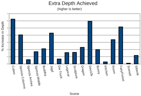
erage increase in depth (see Figure 5). It is important to remember 338
though that a depth increase of one level in the tree has to the po-339
tential to reduce the number of nodes under the entry point by half. 340
Mean extra depth achieved was 2.54% with a standard deviation of 341
1.96%. Maximum extra depth achieved was 6.24%. 342
6.2 Phase 2
343
Phase 2 (returning the best entry point in the candidate list) is scored 344
on its speed to find the entry point. Our results (see Figure 6) in-345
dicate speedups up to 144%, with a mean speedup of 57.68% and 346
a standard deviation of 40.75%. No scene exhibits a slowdown, as 347
predicted in Section 3.2. This is a result of the decreased number of 348
nodes visited due to not needing to scan the entire candidate list. 349
6.3 Overall Performance
350
In order to test the overall performance of our new algorithm, we 351
measure the frames per second achieved by our real-time ray-tracer 352
using basic packet-tracing, MLRTA and AEPSA across our test 353
scene database. Results show an across-the-board gain in render-354
ing speed using AEPSA of up to 36% over packet-tracing and a 355
[image:5.595.322.557.57.218.2]speedup of up to 18% over MLRTA (see Figure 7). 356
Figure 5: Percentage of extra depth achieved over MLRTA. That is,
(Ad−M d)/M d∗100, whereAdandM dare the average depths of the entry points in the kD-Tree returned by the MLRTA and AEPSA algorithms, respectively.
Figure 6: Speedups achieved over MLRTA in finding the entry point
in phase 2. In order to compare the second phase times more ac-curately, we use MLRTA phase 1 for both algorithms. This ensures that both algorithms have the same number of candidate nodes to check and that both algorithms return the same entry point.
7
Discussion
357
Our tests indicate that in certain cases MLRTA is detrimental to 358
rendering speeds. Two scenes, “Jagd” and “DW Truck” exhibit 359
slowdowns under MLRTA. AEPSA shows slowdowns on neither 360
of these scenes. The entry point search time (see Figure 6) for both 361
of these scenes under AEPSA is on the order of one half the time 362
MLRTA takes, indicating that too long of an EP search time can out-363
weigh any benefits gained. In all cases the performance of AEPSA 364
is greater than or equal to the rendering speed exhibited by MLRTA. 365
Using a Pearson Product-Moment Correlation we find no signif-366
icant simple linear correlation between the tree characteristics in 367
table 1 and overall speedup, indicating that if such a correlation 368
[image:5.595.324.561.302.463.2]Figure 7: Using basic packet tracing as a baseline, we compare the
overall performance of our real-time ray-tracer using AEPSA and MLRTA. In all cases AEPSA produces a speedup.
8
Further Work
370
As we use culling techniques in our leaf nodes during the entry-371
point search, it may be beneficial to skew the kD-tree compiler 372
towards creating leaves of larger volume. Such a skewing may 373
make it easier to cull leaf nodes as the ray proxy frustum will be 374
more likely to pass through leaves without intersecting any geome-375
try stored in the node. We intend to investigate tuning tree creation 376
to leverage our algorithm’s strengths. 377
Entry point search algorithms have been used with other accelera-378
tion data structures [Wald et al. 2006]. We intend to investigate the 379
use of AEPSA with bounding volume hierarchies and the bounding 380
interval hierarchy [W¨achter and Keller 2006] [Waechter 2007]. 381
9
Conclusion
382
We have presented a two-phase extension to MLRTA for finding 383
deep entry points in acceleration data structures such as kD-trees 384
or BVHs for real-time ray-tracing. We have compared this algo-385
rithm to the state-of-the-art entry point search algorithm on which 386
we base our work. Our results indicate a decrease in time to find 387
the entry point and an increase in entry point depth across all of our 388
tested scenes. The overall performance of our real-time ray-tracing 389
system showed an increase in frames per second of up to 36%. 390
10
Acknowledgements
391
This section purposely withheld for review purposes. 392
A
AEPSA pseudo-code
393
The following is a simplified implementation using a recursive 394
function to find the candidates. Our actual implemetions of ML-395
RTA and AEPSA are completely iterative functions with software 396
stacks for performance. 397
PROC aepsa(tree, frustum)
398
stack //holds candidates
399
find_candidates(root(tree),
400
frustum, stack)
401
402
WHILE NOT empty(stack) DO
403
node = pop(stack)
404
IF traverse_to_leaf(frustum, n)
405
along path to leaf not taken
406
overlaps non-empty leaf THEN
407
RETURN WITH n
408
ENDIF
409
ENDWHILE
410
411
RETURN WITH NULL
412
ENDPROC
413
414
415
PROC find_candidates(node, frustum, stack)
416
IF node IS leaf THEN
417
i = intersect(frustum, leaf);
418
IF i == TRUE THEN
419
stack.push(node);
420
RETURN WITH i;
421
ENDIF
422
ENDIF
423
424
s = find_candidates(left(node)
425
OR find_candidates(right(node));
426
427
IF s == TRUE THEN
428
push(stack, node)
429
ENDIF
430
ENDPROC
431
References
432
APPEL, A. 1968. Some Techniques for Shading Machine Ren-433
derings of Solids. In AFIPS 1968 Spring Joint Computer Conf., 434
vol. 32, 37–45. 435
BENTHIN, C. 2006. Realtime Ray Tracing on current CPU Ar-436
chitectures. PhD thesis, Computer Graphics Group, Saarland
437
University. 438
COOK, R. L., PORTER, T., ANDCARPENTER, L. 1984. Dis-439
tributed ray tracing. In Computer Graphics (SIGGRAPH ’84 440
Proceedings), vol. 18, 137–45.
441
DMITRIEV, K., HAVRAN, V., ANDSEIDEL, H.-P. 2004. Faster 442
Ray Tracing with SIMD Shaft Culling. Research Report MPI-443
I-2004-4-006, Max-Planck-Institut fr Informatik, Saarbr¨ucken, 444
Germany, December. 445
FOLEY, T., AND SUGERMAN, J. 2005. KD-tree Acceleration 446
Structures for a GPU Raytracer. In HWWS ’05: Proceedings of 447
the ACM SIGGRAPH/EUROGRAPHICS conference on
Graph-448
ics hardware, ACM Press, New York, NY, USA, 15–22.
449
GLASSNER, A. S., Ed. 1989. An introduction to ray tracing. Aca-450
demic Press Ltd., London, UK, UK. 451
HAVRAN, V.,ANDBITTNER, J. 2000. Lcts: Ray shooting using 452
longest common traversal sequences. In Proceedings of Euro-453
graphics (EG’00), 59–70.
454
HAVRAN, V. 2000. Heuristic Ray Shooting Algorithms. Ph.d. the-455
sis, Department of Computer Science and Engineering, Faculty 456
of Electrical Engineering, Czech Technical University in Prague. 457
HAVRAN, V., 2005. On The Kd-tree Construc-458
tion Algorithms with Surface Area Heuristics.
459
HORN, D. R., SUGERMAN, J., HOUSTON, M.,ANDHANRAHAN, 461
P. 2007. Interactive k-d Tree GPU Raytracing. In I3D ’07: 462
Proceedings of the 2007 symposium on Interactive 3D graphics
463
and games, ACM Press, New York, NY, USA, 167–174.
464
HURLEY, J., KAPUSTIN, A., RESHETOV, A.,ANDSOUPIKOV, A. 465
2002. Fast Ray Tracing for Modern General Purpose CPU. In 466
Proceedings of GraphiCon 2002.
467
INTEL. 2006. Intel 64 and IA-32 Architectures Software Devel-468
oper’s Manual Volume 2B: Instruction Set Reference, N-Z. ch. 4,
469
246–247. 470
MACDONALD, D. J.,ANDBOOTH, K. S. 1990. Heuristics for ray 471
tracing using space subdivision. Vis. Comput. 6, 3, 153–166. 472
RESHETOV, A., SOUPIKOV, A., ANDHURLEY, J. 2005. Multi-473
level ray tracing algorithm. In SIGGRAPH ’05: ACM SIG-474
GRAPH 2005 Papers, ACM Press, New York, NY, USA, 1176–
475
1185. 476
RESHETOV, A. 2006. Omnidirectional ray tracing traversal algo-477
rithm for kd-trees. In In Proceedings of the IEEE Symposium on 478
Interactive Ray Tracing, pages, 57–60.
479
RESHETOV, A. 2007. Faster ray packets - triangle intersection 480
through vertex culling. In SIGGRAPH ’07: ACM SIGGRAPH 481
2007 posters, ACM, New York, NY, USA, 171.
482
STANFORD. The Stanford 3d scanning repository. 483
http://graphics.stanford.edu/data/3Dscanrep. 484
W ¨ACHTER, C., ANDKELLER, A. 2006. Instant Ray Tracing: 485
The Bounding Interval Hierarchy. In Rendering Techniques 486
2006 (Proc. of 17th Eurographics Symposium on Rendering),
487
T. Akenine-M¨oller and W. Heidrich, Eds., 139–149. 488
WAECHTER, C. 2007. Quasi-Monte Carlo light transport simula-489
tion by efficient ray tracing. Ph.d. thesis, University of Ulm.
490
WALD, I., BENTHIN, C., WAGNER, M., AND SLUSALLEK, P. 491
2001. Interactive rendering with coherent ray tracing. In 492
Computer Graphics Forum (Proceedings of EUROGRAPHICS
493
2001, Blackwell Publishers, Oxford, A. Chalmers and T.-M.
494
Rhyne, Eds., vol. 20, 153–164. available at graphics.cs.uni-495
sb.de/ wald/Publications. 496
WALD, I., IZE, T., KENSLER, A., KNOLL, A., AND PARKER, 497
S. G. 2006. Ray tracing animated scenes using coherent grid 498
traversal. In SIGGRAPH ’06: ACM SIGGRAPH 2006 Papers, 499
ACM Press, New York, NY, USA, 485–493. 500
WALD, I. 2004. Realtime Ray Tracing and Interactive Global 501
Illumination. PhD thesis, Computer Graphics Group, Saarland
502
University. 503
WHITTED, T. 1980. An improved illumination model for shaded 504