Luis Fabricio Guamán Guevara
A Thesis Submitted for the Degree of PhD
at the
University of St Andrews
2019
Full metadata for this thesis is available in
St Andrews Research Repository
at:
http://research-repository.st-andrews.ac.uk/
Please use this identifier to cite or link to this thesis:
http://hdl.handle.net/10023/17792
This item is protected by original copyright
This item is licensed under a
Creative Commons License
Luis Fabricio Guamán Guevara
This thesis is submitted in partial fulfilment for the degree of
Doctor of Philosophy (PhD)
at the University of St Andrews
ii
I, Luis Fabricio Guaman Guevara, do hereby certify that this thesis, submitted for the degree of PhD, which is approximately 53,000 words in length, has been written by me, and that it is the record of work carried out by me, or principally by myself in collaboration with others as acknowledged, and that it has not been submitted in any previous application for any degree.
I was admitted as a research student at the University of St Andrews in November 2014.
I received funding from an organisation or institution and have acknowledged the funder(s) in the full text of my thesis.
Date Signature of candidate
Supervisor's declaration
I hereby certify that the candidate has fulfilled the conditions of the Resolution and Regulations appropriate for the degree of PhD in the University of St Andrews and that the candidate is qualified to submit this thesis in application for that degree.
Date Signature of supervisor
Permission for publication
In submitting this thesis to the University of St Andrews we understand that we are giving permission for it to be made available for use in accordance with the regulations of the University Library for the time being in force, subject to any copyright vested in the work not being affected thereby. We also understand, unless exempt by an award of an embargo as requested below, that the title and the abstract will be published, and that a copy of the work may be made and supplied to any bona fide library or research worker, that this thesis will be electronically accessible for personal or research use and that the library has the right to migrate this thesis into new electronic forms as required to ensure continued access to the thesis.
iii
Printed copy
No embargo on print copy.
Electronic copy
No embargo on electronic copy.
Date Signature of candidate
iv
I, Luis Fabricio Guaman Guevara, hereby certify that no requirements to deposit original research data or digital outputs apply to this thesis and that, where appropriate, secondary data used have been referenced in the full text of my thesis.
v
The global ocean has experienced an alteration of its seawater chemistry due to the
continuing uptake of anthropogenic carbon dioxide (CO2) from the atmosphere. This
ongoing process called Ocean acidification (OA) has reduced seawater pH levels,
carbonate ion concentrations (CO3-2) and carbonate saturation state (Ω) with
implications for the diversity and functioning of marine life, particularly for marine
calcifiers such as foraminifera.
The vulnerability of this ubiquitous calcifying group to future high pCO2 /low pH
scenarios has been assessed naturally and experimentally in the last decades. However,
little is known about how benthic foraminifera from coastal environments such as
intertidal environments will respond to the effects of OA projected by the end of the
century.
This research aimed to quantify the effects of OA on a series of biological parameters
measured on the benthic foraminifera Elphidium williamsoni and Haynesina germanica
through a laboratory-based experimental approach where future scenarios of a high CO2
atmosphere and low seawater pH were explored.
Experimental evidence revealed that survival rates, test weight and size-normalized
weight (SNW) of E. williamsoni were negatively affected by OA. Whereas H.
germanica was positively affected (i.e. enhanced growth rates) showing a
species-specific response to OA at 13°C. However, the combined effect of OA and temperature
(15°C) reduced survival and growth rates for Elphidium williamsoni and Haynesina
vi
uptake of 13C-labelled diatoms of Navicula sp., notably for E. williamsoni.
Test dissolution rates were enhanced by OA and negatively affected foraminiferal
morphology of recently dead assemblages with implications for net accumulation and
preservation. These results imply that the long-term storage of inorganic carbon and
cycling of carbon in coastal benthic ecosystems will be considerably altered by future
vii
First of all, I would like to thank my supervisor Prof. Bill Austin and Dr Richard
Streeter for your guidance and friendship throughout this 4-year learning process. Their
continuous support and advice encouraged me to become an exceptional person and
independent professional on a research area totally unknown before the onset of this
PhD programme.
I am also grateful to Dr Heather Austin for her patience and knowledge provided at the
start of the experimental period in 2015. Her invaluable expertise and help were
fundamental to fulfil all research goals.
I would also like to thank Prof. David Paterson, Andrew Blight and Irvine Davidson for
providing me with an excellent and cosy working place in the premises of
Sediment Ecology Research Group (SERG) at the Scottish Oceanographic Institute
(SOI). To Jack, Ben, Adam, Joe, Julie and everyone else from the SERG Group who
with a simple but warm conversation during coffee/tea breaks exceptionally inspired
and encouraged me to complete my long journeys of laboratory work.
I am especially thankful to Dr Natalie Hicks from The Scottish Association for Marine
Science (SAMS) who was acting as external supervisor and actively supporting my
research from the beginning of my PhD programme. Furthermore, I highly appreciate
her continuous support, valuable comments and suggestions at every stage of this study.
Her contagious joy and optimism made me feel like I was at home again. Dr Natalie
Hicks and Dr Tim Brand gave me an extraordinary opportunity to spend some time at
viii
Also, I would like to express my sincere gratitude to Fiona Müller-Lundin and
Gunasekaran Kannan for their continuous interest and valuable contribution to this
present research. I feel so honoured to have had the opportunity of supervising their
independent researches and also fortunate for getting to know extraordinary persons,
colleagues and friends who will always stand out anywhere they are pursuing other
personal or academic goals.
I am especially thankful to Dr Emilia Ferraro whom by causality I met her in Ecuador
during the UK Universities fair and who became my first contact encouraging me to
apply to a PhD programme in the School of Geography and Sustainable Development at
the University of St Andrews. Thanks for all the encouragement and help received.
Especial thanks to everyone who I have met within and outside of the School of
Geography and Sustainable and Development throughout these four years of personal
and professional challenges. Thanks for giving me the opportunity of learning a new
football style and contribute with an extensive number of goals. By doing this activity
and Aikido I re-discovered my own talents and strength, but most important thing was
to recognize that not only talent is required to become a better player or researcher but
also hard-working, passion, determination, motivation, patience and collective work are
constantly needed.
I am also grateful to the staff of English Language Teaching at the University of St
Andrews who continuously provided me high-quality foundations to success in this PhD
ix
pleasant and friendly working environment at School of Geography and Sustainable and
Development and School of Earth and Environmental Sciences. In addition, I would like
to thank all the people I have met over the last 4 years being part of Dr Bill Austin’s
group.
Finally, especial thanks to Ranald Strachan (Fife Countryside Ranger for the Eden
Estuary) and Gavin Johnson, both from Fife Coast and Countryside Trust, and Scottish
National Heritage, for their permanent support and for permitting the sampling on Eden
Estuary.
This thesis would have never been finished without a continuous and unconditional
support of my family which in spite of distances and time differences have always been
here and now with me.
Funding
This work was supported by the National Institution of Higher Education, Science,
x
Abstract ... v
General acknowledgements ... vii
Funding ... ix
Table of Contents ... x
List of Figures ... xii
List of Tables ... xvii
Chapter 1. Introduction ... 1
1.1 Coastal Areas ... 1
1.2 Ocean Acidification ... 2
1.3 Carbonate system in an acidifying ocean ... 3
1.4 Evidence of the effect of OA in marine organisms and environments ... 6
1.5 Benthic communities and optimal environmental conditions ... 9
1.6 Introduction to Foraminifera ... 11
1.7 Benthic Foraminifera ... 12
1.8 Aims of Research... 26
1.9 Thesis Structure ... 28
Chapter 2. Materials and Methods ... 29
2.1 Collection site and sampling ... 29
2.2 Identification and abundance of foraminiferal specimens. ... 30
2.3 Foraminiferal calcein incubations ... 31
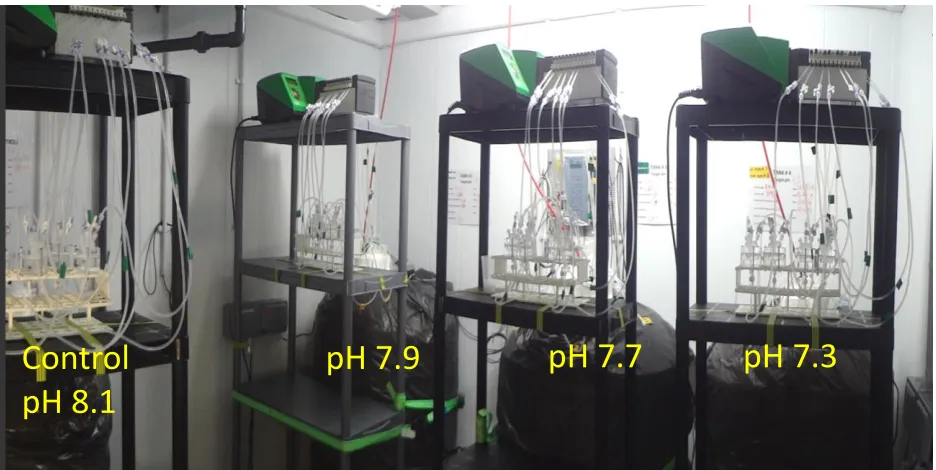
2.4 Culturing chamber setup ... 33
2.5 Carbonate chemistry manipulation system ... 35
2.6 Biological Parameters ... 37
2.7 Foraminiferal feeding ... 42
2.8 Scanning Electron Microscopy (SEM) images ... 44
2.9 Statistical Analysis ... 44
Chapter 3. The effects of short-term high CO2 concentrations and low seawater pH on survival, growth/calcification and taphonomic processes (e.g. dissolution) of the benthic foraminifera E. williamsoni and H. germanica. ... 47
3.1 Introduction ... 47
3.2 Materials and Methods ... 50
3.3 Results ... 55
3.4 Discussion ... 73
xi
4.1 Introduction ... 83
4.2 Materials and Methods ... 86
4.3 Results ... 91
4.4 Discussion ... 112
4.5 Conclusions ... 123
Chapter 5. Feeding efficiency and carbon uptake by benthic foraminifera under Ocean Acidification conditions ... 125
5.1 Introduction ... 125
5.2 Materials and Methods ... 129
5.3 Results ... 141
5.4 Discussion ... 154
5.5 Conclusions ... 162
Chapter 6. The combined effect of increased temperature and elevated CO2 concentration on benthic foraminifera growth and calcification. A case study of two independent laboratory experiments. ... 163
6.1 Introduction ... 163
6.2 Materials and Methods ... 163
6.3 Results ... 172
6.4 Discussion ... 189
6.5 Conclusions ... 198
Chapter 7. Short-term effects of high CO2/ low pH levels on post-mortem dissolution of E. williamsoni and H. germanica... 201
7.1 Introduction ... 201
7.2 Materials and Methods ... 204
7.3 Results ... 211
7.4 Discussion ... 215
7.5 Conclusions ... 223
Chapter 8. Discussion ... 225
8.1 General Discussion ... 225
8.2 Limitations and future work ... 242
8.3 Conclusions ... 248
xii
Figure 2. 1 Sampling site, mudflats on Eden Estuary, Fife, UK. ... 29
Figure 2. 2 Living assemblages of Elphidium williamsoni and Haynesina germanica
observed in sediment samples collected from intertidal mudflats on Eden Estuary, Fife, UK. ... 31
Figure 2. 3 Seawater recirculating system used for calcein incubation. ... 32
Figure 2. 4 Foraminiferal culturing system used for CO2 experiments. ... 34
Figure 2. 5 Foraminiferal culturing system connected to the controlled recirculating seawater system.. ... 36
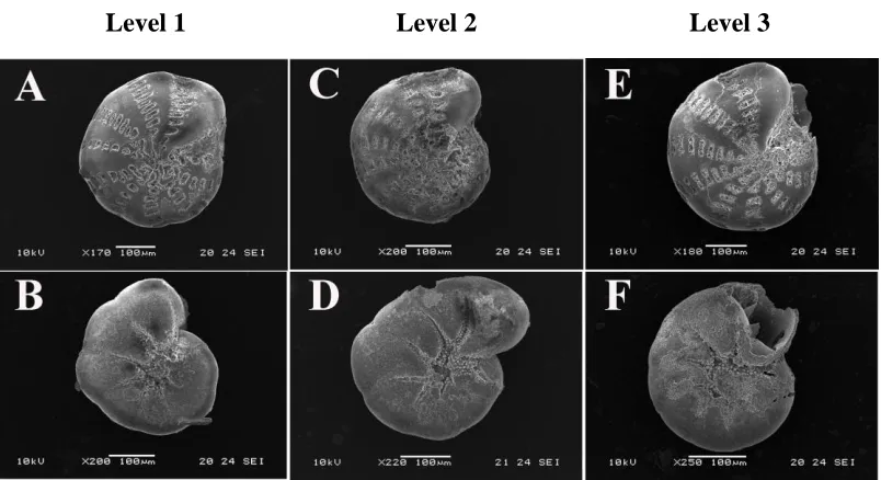
Figure 2. 6 Scanning electron micrographs (SEM) images to illustrate the levels of morphological responses displayed by Elphidium williamsoni and Haynesina germanica
exposed todifferent CO2/pH conditions.. ... 39
Figure 2. 7 Image of live specimens of Elphidium williamsoni and Haynesina germanica displaying new chambers deposited after an experimental period of 31 days at different pH conditions.. ... 40
Figure 3. 1 Calcein incubation of Elphidium williamsoni and Haynesina germanica
under temperature controlled conditions of 13°C for 8 weeks with a light condition of 12:12-hr light: dark cycle.. ... 51
Figure 3. 2 Scanning electron micrographs (SEM) images to illustrate the morphological changes in tests of Elphidium williamsoni observed across pH conditions.. ... 56
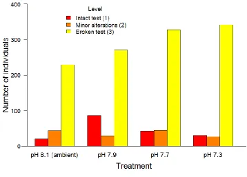
Figure 3. 3 Number of individuals (‘live’ and recently dead) with morphological changes observed in tests of Elphidium williamsoni as a potential response to experimental pH conditions.. ... 57
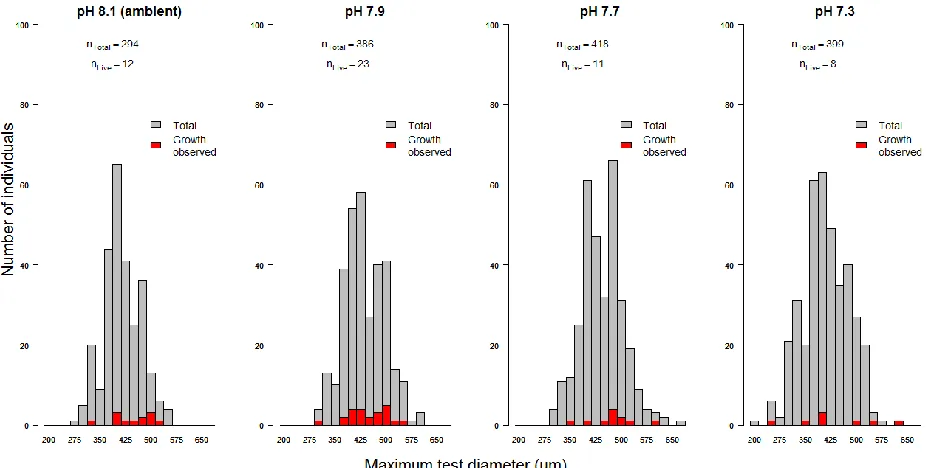
Figure 3. 4 The total number of individuals of Elphidium williamsoni sorted into size classes after being collected at the end of the experimental period in each culture condition (pH 8.1 (ambient), pH 7.9, pH 7.7 and pH 7.3)... 59
Figure 3. 5 Mean values (± standard error) of maximum test diameter (µm) for ‘live’
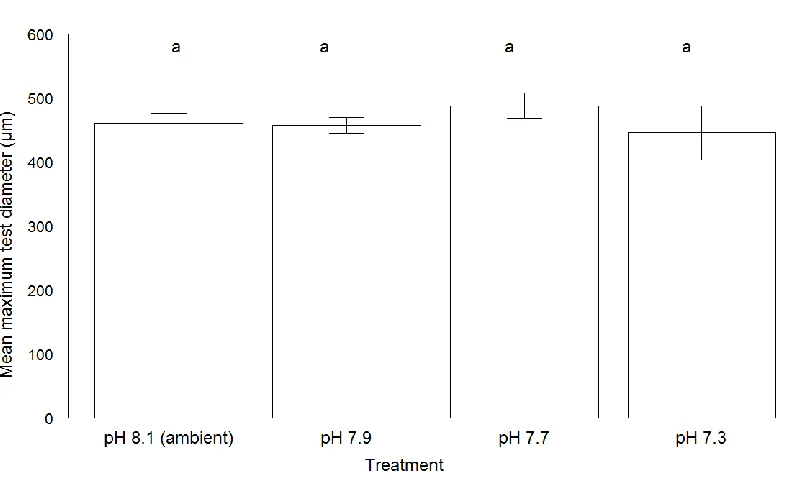
Elphidium williamsoni cultured at different pH conditions.. ... 61
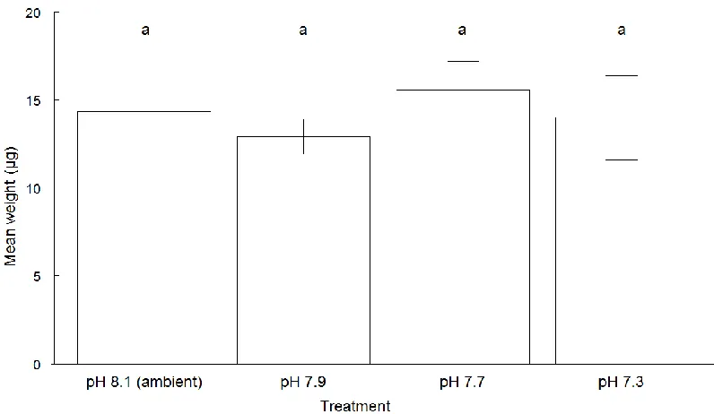
Figure 3. 6 Mean values (± standard error) of weight (µg) for ‘live’ Elphidium williamsoni cultured at different pH conditions ... 63
xiii
Figure 3. 9 Scanning electron micrographs (SEM) of ‘live’ Elphidium williamsoni
cultured at pH 8.1, pH 7.9, pH 7.7 and pH 7.3.. ... 69 Figure 3. 10 Regression line of the relationship between maximum test diameter and test weight for ‘live’ and recently dead Elphidium williamsoni cultured under different experimental pH conditions. ... 72
Figure 4. 1 Seawater recirculating system used for calcein incubation of Elphidium williamsoni and Haynesina germanica under controlled conditions of 13°C for 5 weeks with a light condition of 12:12-hr light: dark cycle.. ... 88
Figure 4. 2 Number of individuals (live and dead) with morphological changes observed in test of Elphidium williamsoni and Haynesina germanica as a potential response to experimental pH conditions.. ... 93
Figure 4. 3 The total number of individuals of Elphidium williamsoni and Haynesina germanica sorted into size classes after being collected at the end of the experimental period from each culture condition (pH~8.1 (ambient), pH 7.9, pH 7.7 and pH 7.3).. .. 95
Figure 4. 4 Distribution of ‘live’ Elphidium williamsoni in relation to maximum test diameter, test weight and number of chambers added for each culture condition (pH 8.1 (ambient), pH 7.9, pH 7.7 and pH 7.3).. ... 98
Figure 4. 5 Distribution of ‘live’ Haynesina germanica in relation to maximum test diameter, test weight, and number of chambers added for each culture condition (pH 8.1 (ambient), pH 7.9, pH 7.7 and pH 7.3).. ... 99
Figure 4. 6 Mean values (± standard error) of maximum test diameter (µm) for live
Elphidium williamsoni and Haynesina germanica cultured at different pH conditions.. ... 101
Figure 4. 7 Mean values (± standard error) of weight (µg) for live Elphidium williamsoni and Haynesina germanica cultured at different pH conditions.. ... 102
Figure 4. 8 Mean values (± standard error) of newly formed chambers for Elphidium williamsoni and Haynesina germanica cultured at different pH conditions.. ... 104
Figure 4. 9 Mean values (± standard error) of mean growth rates for Elphidium williamsoni and Haynesina germanica cultured for 52 days at different pH conditions.
... 106
Figure 4. 10 Mean values (± standard error) of size-normalized test weight (SNW) for
xiv
Figure 4. 12 Scanning electron micrographs (SEM) images of ‘live’ specimens of
Haynesina germanica cultured at pH 8.1, pH 7.9, pH 7.7 and pH 7.3.. ... 111
Figure 4. 13 Regression lines of the relationship between maximum log test diameter and log test weight of Elphidium williamsoni and Haynesina germanica cultured under different experimental pH conditions ... 118
Figure 4. 14 Relationship between mean values (± standard error) of seawater [CO32-]
and size-normalized weight (SNW) for Elphidium williamsoni and Haynesina germanica cultured at different pH conditions. ... 120
Figure 5. 1 Controlled recirculating seawater system used for CO2 experiments. Elphidium williamsoni and Haynesina germanica cultured in natural sediment under controlled conditions of 13°C for 52 days with a light condition of 12:12-h light: dark cycle ... 131
Figure 5. 2 Schematic diagram of the feeding experiment design with 4 pH treatments. Specimens of E. williamsoni and H. germanica were fed once with 13C enriched diatom
Navicula sp.. ... 136
Figure 5. 3 Comparison of carbon isotope ratios (δ13C) of cytoplasm samples of preconditioned Elphidium williamsoni after feeding experiments.. ... 144
Figure 5. 4 Comparison of carbon isotope ratios (δ13C) of cytoplasm samples of preconditioned Haynesina germanica after feeding experiments ... 145
Figure 5. 5 Comparison of individual uptake of phytodetrital carbon (pC) by preconditioned Elphidium williamsoni for 3 hours (T1) (blue) and 72 hours (T2) (red)
after the start of feeding experiment. ... 149
Figure 5. 6 Comparison of individual uptake of phytodetrital carbon (pC) by preconditioned Haynesina germanica for 3 hours (T1) after the start of the feeding
experiment. ... 150
Figure 5. 7 Comparison of individual uptake rates of phytodetrital carbon (pC) by preconditioned Elphidium williamsoni for 3 hours (T1) and 72 hours (T2) after the start
of feeding experiment.. ... 152
Figure 5. 8 Comparison of individual uptake rates of phytodetrital carbon (pC) by preconditioned Haynesina germanica for 3 hours (T1) after the start of the feeding
xv
Figure 6. 2 The total number of individuals of Elphidium williamsoni and Haynesina germanica sorted into size classes after being collected at the end of the experimental period from each culture condition (pH~8.1 (ambient), pH 7.7 and pH 7.3) ... 175
Figure 6. 3 Distribution of ‘live’ Elphidium williamsoni in relation to maximum test diameter, test weight and number of chambers added for each culture condition (pH 8.1 (ambient), pH 7.7 and pH 7.3). ... 177
Figure 6. 4 Distribution of ‘live’ Haynesina germanica in relation to maximum test diameter, test weight and number of chambers added for each culture condition (pH 8.1 (ambient), pH 7.7 and pH 7.3) ... 178
Figure 6. 5 Mean values (± standard error) of maximum test diameter (µm) for ‘live’
Elphidium williamsoni and Haynesina germanica cultured at different pH conditions.. ... 180
Figure 6. 6 Mean values (± standard error) of weight (µg) for Elphidium williamsoni
and Haynesina germanica cultured at different pH conditions. ... 181
Figure 6. 7 Mean values (± standard error) of newly formed chambers for Elphidium williamsoni and Haynesina germanica cultured at different pH conditions. ... 183
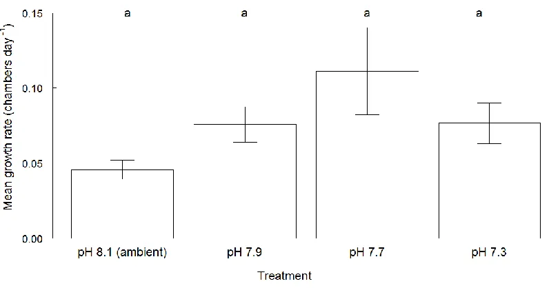
Figure 6. 8 Mean values (± standard error) of mean growth rates (chambers day-1) for
Elphidium williamsoni and Haynesina germanica cultured at different pH conditions. ... 184
Figure 6. 9 Mean values (± standard error) of Size-Normalized test Weight (SNW) for
Elphidium williamsoni and Haynesina germanica cultured at different pH conditions.. ... 185
Figure 6. 10 Scanning electron micrographs (SEM) images of ‘live’ specimens of
Elphidium williamsoni cultured at pH 8.1, pH 7.7 and pH 7.3 ... 186
Figure 6. 11 Scanning electron micrographs (SEM) images of ‘live’ specimens of
Haynesina germanica cultured at pH 8.1, pH 7.7 and pH 7.3. ... 188
Figure 6. 12 Mean values (± standard error) of maximum test diameter (µm) for ‘live’
Elphidium williamsoni and Haynesina germanica cultured at different pH (8.1, 7.7 and 7.3 units) and temperature (13 and 15°C) levels. ... 192
xvi
Figure 7. 1 Schematic diagram of dissolution experiment design for three pH scenarios.. ... 206 Figure 7. 2 Dissolution rates of pre-conditioned and recently dead specimens of
Elphidium williamsoni and Haynesina germanica exposed for a period of 42 days to different experimental pH conditions at 15°C. ... 212
Figure 7. 3 Mean values (± standard deviation) of dissolution rates (µg day-1) for
Elphidium williamsoni and Haynesina germanica exposed for 42 days to different experimental pH conditions at 15°C. ... 213
Figure 7. 4 Scanning electron micrographs (SEM) images to illustrate the level of morphological responses displayed by dead Elphidium williamsoni and Haynesina germanica exposed for 42 days todifferent CO2/pH conditions. ... 214
Figure 7. 5 Estimations of net carbonate productivity (g m-2 year-1) and gross carbonate dissolution (g m-2 year-1, in red) for Elphidium williamsoni and Haynesina germanica
xvii
Table 3. 1 Seawater measurements taken from the experimental carbonate chemistry manipulation system.. ... 55
Table 3. 2 Survival rates (SR) of Elphidium williamsoni and Haynesina germanica
cultured for 31 days under different pH condition ... 58
Table 3. 3 Maximum test diameter (µm) of ‘live’ Elphidium williamsoni cultured under different experimental pH conditions ... 60
Table 3. 4 Test weight of ‘live’ Elphidium williamsoni cultured under different experimental pH conditions ... 62
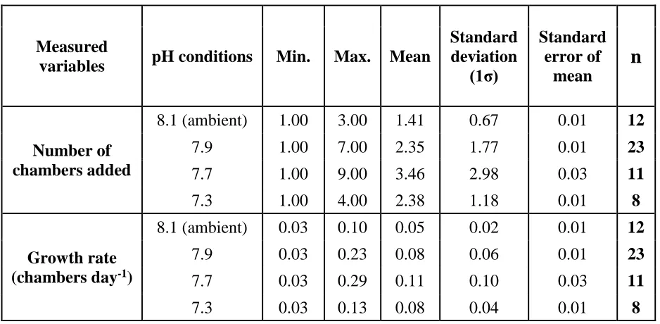
Table 3. 5 Number of chambers added and growth rate of ‘live’ Elphidium williamsoni
cultured under different experimental pH conditions ... 64
Table 3. 6 Comparison between slopes of the linearised function defining the relationship between maximum diameter and test weight for ‘live’ Elphidium williamsoni cultured under different experimental pH conditions ... 67
Table 3. 7 Comparison between slopes of the relationship between maximum diameter and test weight for ‘live’ and recently dead Elphidium williamsoni cultured under different experimental pH conditions ... 71
Table 4. 1 Average seawater measurements taken fortnightly from carbonate chemistry manipulation system ... 91
Table 4. 2 Survival rates (SR) of Elphidium williamsoni and Haynesina germanica
cultured for 52 days under different pH conditions ... 94
Table 4. 3 Maximum test diameter, weight and new chambers added to live Elphidium williamsoni and Haynesina germanica cultured for 52 days under different experimental pH conditions. ... 96
Table 4. 4 Mean growth rates based on the number of chambers added by Elphidium williamsoni and Haynesina germanica cultured for 52 days under different experimental pH conditions. ... 105
Table 5. 1 Average seawater measurements taken fortnightly from carbonate chemistry manipulation system ... 141
xviii
Table 5. 4 Two-way ANOVA to compare the effects of the time period and pH treatments on dependent variable pC (content of phytodetrital carbon) mainly in
Elphidium williamsoni cultured under different experimental pH conditions ... 148
Table 5. 5 Two-way ANOVA to compare the effects of the time period and pH treatments on dependent variable carbon uptake rate mainly by Elphidium williamsoni
cultured under different experimental. ... 151
Table 6. 1 Seawater measurements taken fortnightly from the experimental carbonate chemistry manipulation system.. ... 172
Table 6. 2 Survival rates (SR) of Elphidium williamsoni and Haynesina germanica
cultured for 52 days under different pH conditions: pH~8.1 (ambient), pH 7.7 and pH 7.3. ... 174
Table 6. 3 Maximum test diameter, weight and new chambers added of ‘live’ Elphidium williamsoni and Haynesina germanica cultured under different experimental pH
conditions: pH~8.1 (ambient), pH 7.7 and pH 7.3. ... 176
Table 7. 1 Estimates of mean dissolution rates (µg day-1) for two dominant calcareous
1
Chapter 1
.
Introduction1.1 Coastal Areas
Coastal zones account for approximately 10% of the ocean area and include coastal
waters and the adjacent shorelands. These marine areas comprise a wide range of
ecosystems such as intertidal areas, salt marshes, wetlands, mudflats, mangroves forests,
coral reefs, sandy beaches and rocky shores ( Lalli & Parsons 1997; Mitra et al. 2014;
Parsons et al. 2016). Although these coastal areas are considered as some of the most
productive and biologically diverse in the world (Solan et al. 2004); due to their
proximity to land, the ecosystem services provided by these marine habitats are strongly
influenced by anthropogenic factors such as eutrophication, overfishing, pollution and
habitat destruction ( Solan et al 2004; Lalli & Parsons 1997; Halpern 2008; Lopes et al
2015; Brouwer et al. 2016). In addition, these areas are also potentially vulnerable to
global threats such as global warming, sea level rise and ocean acidification (OA) that
might have additional consequences for these marine ecosystems (Morton et al. 2011;
IPCC 2013; Strong et al. 2014; Parsons et al. 2016). For instance, notable changes in
biological productivity caused by the alteration of biogeochemical cycling of carbon
and nutrients, biodiversity reduction and loss of natural habitats are expected as direct
responses of coastal habitats to these environmental factors (Solan et al. 2004).
These multiple stressors might have the potential for synergistic, additive or cumulative
effects on coastal environments (Boyd & Hutchins 2012). This environmental
complexity supports the need for laboratory experiments to unravel the effects of
2
associated impact on marine ecosystems and productivity on local and global scales
(Murray 2006; Horton & Murray 2007).
1.2 Ocean Acidification
Anthropogenic activities such as fossil-fuel combustion, deforestation, agriculture, industrialization, cement production and changes in land-use have caused a steady increase in atmospheric CO2 concentrations since industrial revolution times. The
subsequent absorption of part of this CO2 by the ocean (~30% of total CO2 emissions)
has changed seawater chemistry through a process known as ocean acidification (OA)
(Caldeira & Wickett 2003; Sabine 2004; Guinotte & Fabry 2008; Keul et al. 2013). As a
result of this process, seawater pH, carbonate ion concentration [CO32-], and saturation
state (Ω) with respect to carbonate minerals have been declining (Gattuso et al. 1998;
Langdon et al. 2000; Caldeira & Wickett 2003; Feely et al. 2004; Sabine 2004; Raven et
al. 2005).
Since the pre-industrial period until the present time, the concentration of CO2 in the
atmosphere has been steadily increased from 280 parts per million (ppm) to exceed 400
ppm by volume (ppmv) (Raven et al. 2005; Guinotte & Fabry 2008; Betts et al. 2016).
However, model predictions (IS92a CO2 emission scenario) by the Intergovernmental
Panel on Climate Change (IPCC) suggest that these levels may exceed 1000 ppmv by
the end of the year 2100 unless considerable reductions in future CO2 emissions occur.
Hence, estimatedrates of increase in CO2 concentrationsin theatmosphere over the next
centuries may be 100 times faster than the maximum rate observed in at least the past
3
Although the reduction in the ocean pH is mainly linked to atmospheric CO2 uptake, the
atmospheric deposition of other chemicals such as nitrogen, and sulphur can also
change the surface ocean chemistry (Guinotte & Fabry 2008; Gattuso & Hansson 2011).
However, these alterations account for only a small proportion of the acidification
compared to the anthropogenic CO2 uptake by the ocean (Doney et al. 2007; Gattuso &
Hansson 2011).
It is estimated that the current seawater pH value has already dropped by 0.1 pH units
over the last two centuries (Orr et al. 2005). This implies an increase in both hydrogen
ion concentration [H+] and its corresponding acidity levels in seawater of approximately 30% in comparison with preindustrial values. Projected ocean pH values indicate an
additional drop of 0.3–0.4 and 0.77 pH units by the year 2100 and 2300, respectively
(Gattuso et al. 1998; Caldeira et al. 2003; Orr et al. 2005; Raven et al. 2005; Caldeira et
al. 2007; Feely et al. 2008; Guinotte & Fabry 2008; Gattuso & Hansson 2011; Tyrrell
2011; IPCC 2013). Changes in the natural seawater pH levels projected for the year
2100 may represent an event not recorded on Earth’s history in at least the past 20
million years (Feely et al. 2004).
1.3 Carbonate system in an acidifying ocean
Through the continuous air-sea gas exchange, atmospheric CO2 is taken up by the upper
ocean to form carbonic acid (H2CO3) with an immediate dissociation to form
bicarbonate ions (HCO3−) and carbonate ions (CO32−) (see Equation 1.1). The equilibria
between carbonate species in the ocean are briefly detailed as follows (see Equation 1.1)
(Zeebe & Wolf-Gladrow 2001; Tyrrell 2011):
4
In seawater, as the concentrations of H2CO3 and CO2 (aq.) are really small, the sum of
their concentrations is often represented as[CO2] (see Equation 1.2).
[CO2] = [CO2 (aq.)] + [H2CO3] (Eq. 1.2)
Where brackets represent total stoichiometric concentrations.
Thus, the concentrations of the three dissolved carbonate species account for: [HCO3−]
(>86.5%), followed by [CO32−] (13%) and [CO2] (~0.5 %) (Zeebe & Wolf-Gladrow
2001). As a consequence of the equilibria among the three carbonate species, seawater
is weakly buffered with respect to changes in hydrogen ion concentration [H+].
The three carbonate species are collectively referred to as Dissolved Inorganic Carbon
(DIC) (Tyrrell 2011; Gattuso & Hansson 2011). Most of the CO2 absorbed by the ocean
over the last two centuries not only has increased the DIC content of seawater but also
has increased the release of more H+ while lowering both pH and [CO
32−] availability
(Raven et al. 2005; Tyrrell 2011). Thus, under future scenarios of an increase in CO2
(aq.) concentrations in seawater, a higher H+ will consume more [CO32−] available to
form immediately [HCO3−] diminishing the pH buffering capacity of surface ocean
(Raven et al. 2005). Current [CO32−] already exhibits a reduction in the availability of
approx. 30%, and it is estimated that this amount will increase in the next centuries
more likely affecting the productivity of the oceans through a decrease in CaCO3
production (Gattuso & Hansson 2011).
The process of formation and dissolution of carbonate minerals are strongly related to
marine photosynthesis and respiration (organic matter oxidation). To some extent, all
processes together control the seawater pH and atmospheric CO2 concentrations (see
5
→ Biomineralization Photosynthesis
Ca2+ + 2HCO3− ⇔ CaCO3 + CO2 + H2O ⇔ CaCO3 + CH2O + O2 (Eq. 1.3)
Dissolution Respiration ←
The formation of carbonate minerals (calcification) takes place when the reaction moves
to the right and is commonly described by Eq. 1.3. The calcification process is nearly all
biogenic, and in the absence of photosynthesis, the biomineralization releases CO2 back
to the atmosphere. Thus, a potential decline in calcification rates may increase the CO2
storage capacity in the upper oceans exerting a negative feedback on atmospheric CO2
levels with ultimate opposing effects on the marine carbon cycle (Riebesell et al. 2000;
Feely et al. 2004). In contrast, carbonate dissolution process takes place through a
reverse reaction in Eq. 3 (moving to the left side of the equation). This dissolution of
carbonate minerals occurs mainly in the deeper water and on the ocean floor (Erez
2003).249
Seawater is in an equilibrium state when the saturation state of carbonate minerals (Ω)
is equal to 1; dissolution of CaCO3 minerals occurs in undersaturated seawater when Ω
is lower than 1, whereas inorganic precipitation takes place in supersaturated seawater
at Ω greater than 1 (Gattuso & Hansson 2011; Tyrrell 2011). Calcite, aragonite and
magnesium calcite (Mg-calcite) are the most important precipitated carbonate minerals
produced by marine calcifying organisms (Gattuso & Hansson 2011; Orr et al. 2005),
and based on their structure, aragonite is more easily dissolved due to its higher
solubility product (K∗sp) and lower saturation state compared with calcite (Ω ar < Ω ca).
The availability and stability of carbonate minerals are affected by the concentration of
6
calcifiers from colder and more acidic waters due to a greater amount of dissolved CO2
may be more affected than calcifiers from warmer waters (Guinotte & Fabry 2008).
The calcium carbonate saturation state (Ω) for carbonate minerals is the determining
factor in the kinetics of precipitation or dissolution of CaCO3, and it is defined as the
ratio between the observed ion product and the expected ion product when the solution
is in equilibrium with particular calcium carbonate mineral (see Equation 1.4):
Ω = [Ca2+] × [CO
32−] / K∗sp (Eq. 1.4)
Owing to [Ca2+] and K∗
sp being relatively constant through the oceans, variations of Ω
are driven mainly by [CO32−]. K*sp represents the solubility product of a specific
carbonate mineral phase at in situ temperature, salinity and pressure (Zeebe &
Wolf-Gladrow 2001; Dueñas-bohórquez et al. 2011)
In general, an important reduction in both [CO32−] and calcium carbonate saturation
state (Ω) may have deleterious consequences mainly for marine biota that rely on
biogenic carbonate minerals to build up their skeletons (Orr et al. 2005).
1.4 Evidence of the effect of OA on marine organisms and environments
Certainly, the amount of atmospheric CO2 absorbed by the ocean has helped mitigate
global climatic impacts (Sabine 2004; Fabry et al. 2008; Dissard et al. 2010; Gattuso &
Hansson 2011). However, this process of CO2 uptake has changed the carbonate
chemistry of seawater causing a wide range of effects on marine environments and
associated biota, particularly on marine organisms with CaCO3 structures. The
7
last two centuries will make it more difficult for calcifiers to be efficiently adapted to
cope with these changes over the next centuries (Guinotte & Fabry 2008).
Although the effects of OA are much better understood, there is still a limited
understanding of the implications of OA across different marine ecosystems (Benjamin
S. Halpern, Shaun Walbridge, Kimberly A. Selkoe et al. 2008).Most of the evidence to
date about the effects of OA comes from in-situ and laboratory experiments on
calcifying organisms from two different trophic levels: primary producers (e.g.
coccolithophores, coralline algae, etc.) (Kuffner et al. 2008; Beaufort et al. 2011; Porzio
et al. 2018), and secondary consumers (e.g. corals, foraminifers, pteropods, mussels and
oysters) (Moodley et al. 2000; Ries 2011; Feely et al. 2004; Maier et al. 2012; Allison et
al. 2010; Allison et al. 2011; Keul et al. 2013; Kuroyanagi et al. 2009; Khanna et al.
2013; van Dijk et al. 2017). The ultimate findings from these studies are, in some cases,
markedly different from each other due to the natural variability among individuals,
developmental stage, taxonomic groups, species, communities, ecosystems and
experimental exposure time (Raven et al. 2005; Zeebe et al. 2008; Bernhard et al. 2009;
Keul et al. 2013; Kroeker et al. 2013).
In general, previous research, although with some exceptions exhibiting a positive or no
influence of OA on survival, growth and calcification of marine organisms
(Iglesias-Rodriguez et al. 2008; Ries et al. 2009; Kroeker et al. 2010; Kroeker et al. 2011; Hikami
et al. 2011; Rodolfo-Metalpa et al. 2011; Vogel & Uthicke 2012; Kroeker et al. 2013;
McIntyre-Wressnig et al. 2013; McIntyre-Wressnig et al. 2014; Connell et al. 2017;
Doubleday et al. 2017), the decline in calcification efficiency due to a reduction in
8
of marine organisms and ecosystems to adverse effects of OA (Riebesell et al. 2000;
Caldeira & Wickett 2003; Orr et al. 2005; Andersson et al. 2008; Maier et al. 2012;
Kroeker et al. 2013).
For instance, with a decreased calcification in corals and coral reef communities, the
coral distribution and its reef framework may be considerably reduced resulting in a
decline of the overall productivity of reef environments (Gattuso et al. 1998; Kleypas et
al. 2001; Leclercq et al. 2002; Kleypas et al. 2006; Jokiel et al. 2008). As the
calcification process in corals also depends on other factors such temperature, water
depth, light and nutrients, any alteration in calcification rates in corals should not be
exclusively linked to a single environmental forcing such as low pH levels and its
corresponding low [CO32−] (Kleypas et al. 2006).
In other organisms also with carbonate exoskeletons such as pteropods and
foraminifera, a reduced calcification rate may make them particularly vulnerable to
erosion (both biological and physical) and dissolution processes (Orr et al. 2005; Raven
et al. 2005).
Laboratory experiments on coccolithophores, corals and foraminifera have already
shown a reduction in calcification up to 50% when the atmospheric CO2 concentration
was set to two-fold the pre-industrial values (from 280 to 560 ppm CO2) (Feely et al.
2004; Raven et al. 2005; Guinotte & Fabry 2008). This decrease in calcification rates
may continue to decline in pteropods, corals (warm-water corals) and some calcareous
algae possessing aragonite as the main carbonate mineral in their skeletal structures due
9
Under projected scenarios of a high CO2 world, a reduction in calcification rates and an
increase of dissolution rates may considerably affect the competitive fitness of some
calcareous species. This also could lead to a shift in natural communities (e.g. benthic
communities), resulting in an ultimate loss of calcareous species all over the world and
giving more ecological and evolutionary competitive advantage to organism whose
skeletal structures are limited in mass or made of materials other than CaCO3
(non-calcifying organisms) (Bambach et al. 2002; Raven et al. 2005; Fabry et al. 2008;
Kuffner et al. 2008; J. Ries 2011). This fact may reduce the structural complexity of
coastal marine communities by reducing their biodiversity, biological interactions and
productivity (Agostini et al. 2018).
Furthermore, a reduction in surface biogenic CaCO3 production due to higher CaCO3
dissolution rate may cause a substantial decline in the net rate of CaCO3 accumulation
and burial on deep seafloor and shallow waters sediments. The long-term implications
of reduced calcification rates by planktonic and benthic calcifiers associated with future
ocean chemistry changes may affect substantially the amount of material available for
the sedimentation of organic matter and CaCO3, with an ultimate impact on marine
carbon cycle (Wolf-Gladrow et al. 1999; Zeebe & Wolf-Gladrow 2001; Marshall et al.
2013).
1.5 Benthic communities and optimal environmental conditions
The vertical distribution of benthic communities in the marine sediment is highly
stratified, with species-specific distribution patterns (Barnes & Hughes 1988; Raven et
10
be naturally limited to specific sediment layers depending on their tolerance to the
existing environmental conditions (e.g. oxygen concentration, pH, etc.).
The higher density of organisms occurs within the upper layers of sediments (few
centimetres depth) where pH levels, the oxygen and nutrients supply are not limiting
factors for their ecological and biochemical activities (Alve & Bernhard 1995; Raven et
al. 2005). Considering the uppermost layers of sediments possess pH levels closer to the
overlying seawater (Silburn et al. 2017), surface benthic species with high diversity and
abundance but with a relatively restricted mobility and distribution (e.g. foraminifera)
(Gross 2000) may be more susceptible to slight changes in seawater pH driven by OA in
comparison to other active motile groups (e.g. metazoans) (Raven et al. 2005; Bernhard
et al. 2009). Some species of metazoans with high motility (e.g. burrowers) can reside in
microhabitats created deeper in the sediments to tolerate low pH, the oxygen and
nutrients limitation from surroundings. Thus, these large benthic organisms are adapted
to displace continuously through a naturally strong geochemical gradient of
approximately one unit of pH within the first 30 cm of unmixed sediments (Fenchel &
Riedl 1970; Raven et al. 2005).
Studies of sediments off the UK coast indicate that natural changes in pH of 0.5-1.0
units can also take place within the first cm of sediment, with impacts on benthic
organisms which are not yet fully understood (Ostle et al. 2016). These natural
conditions may drastically change as ongoing OA has the potential to affect ecosystems
and biogeochemical processes driven by benthic communities (e.g. foraminifera)
11
1.6 Introduction to Foraminifera
Foraminifera (Order Foraminiferida, Supergroup Rhizaria) are one of the most diverse
groups of heterotrophic unicellular eukaryotes protists comprising around 10,000 extant
species and tens of thousands of fossil taxa (Vickerman 1992; Flakowski et al. 2005).
The foraminiferal cell body, called test (also referred to as shell), comprises of one or
more chambers whose composition consists of particles cemented together
(agglutinated), forming an organic matrix or CaCO3 (mainly calcite over aragonite)
(Gooday 2003; Barras 2008). Thus, foraminifera have been subdivided based on their test’s characteristics: agglutinated, porcellaneous or hyaline (Murray 2006).
This group of calcifying organisms possesses a relatively short lifespan with an
estimated duration of life ranging from 3 months up to 2 years (Murray 1983; Murray
1991; Barras 2008). Their complex life cycles usually involve an alternation of sexual
and asexual generations. Under intense environmental conditions, this cycle can be
altered and asexual reproduction may be more common (Goldstein 1999; Gooday 2003;
Jones 2014). This biological feature of generations changes may explain the distinct
morphological dimorphism observed in tests of many species, including large fossil
forms (Sen Gupta 1999).
The size of foraminifera depends on the taxa, but generally, their size (test diameter) is
likely to range from 38 µm to 1 cm or longer (Wolf-Gladrow 1999; Murray 2006;
Barras 2008; Uthicke et al. 2013).
Foraminifera possess a retractile cytoplasm and a network of a granulo-reticulose
pseudopodia inside of their test (Gooday 2003; Barras 2008; Jones 2014). Pseudopodia
12
functions are to provide attachment, locomotion, protection, building and structuring the
test (Kitazato 1988; Goldstein 1999; Gooday 2003; Barras 2008; Jones 2013). In
addition, pseudopodia are also highly efficient at food-capturing and contribute largely
to the role foraminifera have in decomposing and recycling high rate of organic carbon
within marine habitats (Bernhard & Bowser 1992; Bowser 2002; Mojtahid et al. 2011).
Geographically, foraminifera are considered as ubiquitous groups and their wide
modern distribution include marine and fresh waters (Archibald et al. 2003; du Châtelet
et al. 2004). However, nearly all the foraminifera groups are constrained to marine
environments with a supremacy of foraminiferal taxa in benthic habitats (99%) (Barras
2008). Depending on their life strategies, foraminiferal planktonic and benthic
communities can be found from deep-sea to coastal environments, frequently forming
the major component of meiofaunal biomass (Bernhard & Bowser 1992; Gooday et al.
1992; Moodley et al. 2000; Murray 2006; Mojtahid et al. 2011).
1.7 Benthic Foraminifera
From the estimated number of 10,000 of extant foraminiferal species (Vickerman 1992),
in comparison with planktonic species, benthic species account for the majority of the
modern foraminifera group and possess a much longer geological record (Sen Gupta
1999). Benthic foraminifera highly contribute to the benthic communities biomass and
diversity, mainly in the deep ocean (Gooday et al. 1992; Moodley et al. 2000; Heip et al.
2001). On a global scale, benthic foraminifera contributes with one-third of the
estimated total annual CaCO3 produced by foraminifera (Schiebel 2002; Langer 2008)
and their estimated contribution in shallow waters range from 5 to 30% of carbonate
13
In shallow and deep waters, benthic foraminifera are vertically distributed from the
uppermost layer up to 35 cm deep in the sediment (Moodley & Hess 1992; Bernhard
1993). The shell morphology of some benthic foraminifera species is related to the
vertical microhabitats they usually inhabit such as epifaunal or shallow (upper 2 cm of
sediments), semi-infaunal and deep infaunal (below the upper 2 cm of sediments)
(Corliss 1991; Moodley & Hess 1992; Linke & Lutze 1993; Loubere et al. 1995)
This benthic group of calcifiers plays a fundamental role in the biogeochemical cycle
due to their ability to degrade large amounts of organic matter in the surface sediments.
Their major contribution in the carbon cycle and CaCO3 cycling is through the
production of skeletons with either high-Mg calcite or low-Mg (calcification) (Moodley
et al. 2002; Habura et al. 2005; Nomaki et al. 2005; Mojtahid et al. 2011; Prazeres et al.
2015).
1.7.1 Trophic dynamics and diet of benthic foraminifera
Given their transitional trophic position between microbes and macrofauna, the trophic
interactions of predation or competition of foraminifera with other species depend
exclusively on their feeding strategies such as carnivory, parasitism, bacterivory,
cannibalism and symbiosis (Goldstein 1999; Gooday 2003; Jones 2014). Thus, they
consume organic carbon mainly from diatoms; however, depending on their habitat and
the prevailing environmental conditions, they can also feed on cyanobacteria,
flagellates, algae, algal-derived detritus, other prokaryotes, metazoans and bacterial
communities (Bernhard & Bowser 1992; Gooday et al. 1997; Mojtahid et al. 2011; Lei
et al. 2014). In all feeding strategies, benthic foraminifera use actively their
14
(Lipps 1983; Vickerman 1992; Austin et al. 2005). However, detailed information on
foraminiferal feeding behaviour is limited to one calcareous intertidal species such as H.
germanica. This benthic species actively uses tooth-like test ornamentations (tubercles)
located on the apertural region to crack frustules of large benthic diatom Pleurosigma
angulatum, consequently removing and ingesting all organic contents (i.e. chloroplasts)
via continuous use of pseudopodia networks (Austin et al. 2005). In general,
diatom-derived chloroplasts usually remain active up to several weeks within the cytoplasm of
benthic foraminifera such as H. germanica (Lekieffre et al. 2018; Jauffrais et al. 2018).
Benthic foraminifera are the main food source for many metazoans living on the
seafloor. This foraminiferal ingestion by other microorganisms can be either as a
selective process carried out by polychaetes, gastropods, nematodes and isopods or as
an indirect process accomplished by fish and other sediment filtering species (Murray
2006; Nomaki et al 2008). This indirect or unselective predation on foraminifera,
mainly on juvenile specimens, may be one of the main factors of the high mortality rate
and low standing crops values observed in foraminifera populations (Cearreta 1988).
1.7.2 Controlling factors
Foraminiferal spatial and temporal distribution as well as abundance, morphology,
diversity, growth, reproduction and isotopic composition are mainly controlled by
biological (i.e. predation, nutrients, food (organic matter) availability, etc.) and abiotic
factors such as seawater temperature, salinity, exposure rates, oxygen conditions, water
depth, pH and [CO32-] gradient, and sediment grain size (substrate) (Hohenegger et al.
15
al. 2011; Reymond et al. 2011; Saraswat et al. 2011; Lei et al. 2014; Pettit et al. 2015;
Brouwer et al. 2016; Eder et al. 2016; Enge et al. 2016).
Relative influence of some specific environmental parameters can vary depending on
the habitat; this will play a major role in the control of distribution and density of
benthic foraminiferal assemblages. For instance, in the deep sea, the predator-prey
relationships with other primary and secondary consumers may influence in the
abundance and diversity of foraminiferal which are not limited only by nutrient and
oxygen availability (Murray 2006; Nomaki et al. 2008; Nomaki et al. 2009). In the case
of intertidal zones, factors such as intertidal vegetation type, phosphate and organic
carbon content, proximity of the open sea, percentage of mud, salinity and tidal
exposure (tidal elevation) may strongly influence the foraminiferal distribution and
density (Armynot du Châtelet et al. 2009).
1.7.3 Foraminiferal growth and calcification process
Foraminiferal growth is usually referred to as a change in biomass, test weight, volume,
test size or number of newly deposited chambers throughout their life cycle (Austin
2003; Reymond et al. 2011; Jones 2014; Briguglio & Hohenegger 2014; Eder et al.
2016; van Dijk et al. 2017). Naturally, the growth rates may vary among species and
also between their life stages (e.g. juveniles and adults). For instance, as the metabolism
is weight-dependent, in early developmental stages, smaller specimens have higher
metabolic requirements in comparison with adults specimens (Mahaut et al. 1995; Heip
et al. 2001). Hence, young specimens are able to grow rapidly with a subsequent
16
favourable environmental conditions, individuals may reach their maximum size as well
as their reproductive maturity (Murray 1983; Austin 2003).
In general, the intermittent production of new chambers is directly linked to the
biological process of calcification. Two mechanisms of calcification have been
described, and in both, the formation of a specific space is fundamental to reach the ions
concentration required for this biological process:
1. In the intracellular process observed in the Miliolid group (porcelaneous,
imperforate), intracellular vesicles accumulate the precipitated calcite crystals, then
these calcifying compartments are transported to the site of chamber formation where
the crystals are released and assembled (Bentov & Erez 2006).
2. in situ precipitation observed in calcite-radial foraminifera (e.g. hyaline, lamellar and
perforated species) starts when pseudopodia partially isolate the individual from their
surroundings by creating a specific space covered by a thin organic matrix with the
shape of the new chamber. Subsequently, CaCO3 is precipitated around this organic
layer which acts as a template for biomineralization. Ultimately, the incorporation of
dissolved essential elements such as Ca2+, CO32− and Mg2+ from the surrounding
seawater facilitate the formation process of their CaCO3 tests (calcite or aragonite)
(Goldstein 1999; Erez 2003; Bentov & Erez 2006; Mojtahid et al. 2011; Mewes et al.
2014).
Although the foraminiferal growth process is intrinsically controlled by genetic factors,
changes in environmental factors might strongly alter calcification and growth processes
17
future decreasing pH levels, and as a response to such unfavourable environmental
conditions, foraminifera may need to invest additional energy to calcification resulting
in less energy for other vital metabolic processes. This ‘trade-off’ may impact
considerably on growth rate, calcification efficiency, fitness of the organism and
ultimately affecting the global inorganic carbon cycle (Raven et al. 2005; de Nooijer et
al. 2009; Dueñas-bohórquez et al. 2011).
1.7.4 Ecological importance as a bioindicator
Benthic foraminifera are widely recognized as remarkable ecological indicators due to
their narrow ecological tolerance levels and their corresponding high sensitivity to
environmental changes (du Châtelet et al. 2004; Schönfeld et al. 2012; Strotz 2015;
Brouwer et al. 2016). The environmental disturbances can be recorded on their CaCO3
tests during their short life cycle before becoming microfossils that are remarkably well
preserved in the deep-sea and coastal sedimentary deposits (Gooday 2003).
Initially, these outstanding characteristics have made it possible for foraminifera to be
used as a tool (proxy) for palaeoenvironmental reconstructions of past sea-level
changes, nutrients, pH, and temperature (Horton et al. 1999; Hintz et al. 2004; Ries
2011; Berkeley et al. 2014; Martínez-Botí et al. 2015). Furthermore, many laboratory
studies have also revealed the importance of using living foraminifera as an
experimental bioindicator to observe ecological changes when environmental drivers
such as salinity, temperature, oxygen, and pH are manipulated (Alve & Bernhard 1995;
Kuroyanagi et al. 2009; Allison et al. 2010; Allison et al. 2011a; R. Saraswat et al.
18
These applications have been used as an analogous tool to further palaeoenvironmental
interpretations of foraminiferal fossil assemblages (Berkeley et al. 2007; Benjamin P.
Horton & Murray 2007; Berkeley et al. 2014), and also to estimate future impacts of
increased seawater surface temperature (global warming) and decreasing seawater pH
(ocean acidification) on coastal marine ecosystems and their productivity as mentioned
below.
1.7.5 Evidence of acidified ocean and its impact on benthic foraminifera
Over the last decade, multiple studies have assessed the effects of changes in seawater
chemistry on benthic foraminifera inhabiting different ecosystems, demonstrating that
the biological response of foraminifera to OA varies both among and within
foraminiferal species (also referred to as a species-specific response).
In general, most studies, with some exceptions exhibiting a positive or no influence of
low pH on calcification, growth, survival, fitness (Hikami et al. 2011; Vogel & Uthicke
2012; McIntyre-Wressnig et al. 2013; McIntyre-Wressnig et al. 2014), show that
projected declining pH can strongly influence biometric and morphological features of
foraminiferal test (e.g. thickness, size/diameter, weight, functional feeding structures,
etc.) with an ultimate effect on the growth and net calcification rates and biomass of
benthic foraminifera, especially in shallow water areas (Kuroyanagi et al. 2009; Allison
et al. 2010; Allison et al. 2011; Fujita et al. 2011; Haynert et al. 2011; Hikami et al.
2011; Khanna et al. 2013; Haynert et al. 2014; Prazeres et al. 2015). However, Keul et
al. (2013) emphasized that foraminiferal growth rates and size-normalized weight
(SNW) were affected mainly by low [CO32-] rather than high CO2 concentrations in
19
Much of this research has focused on the use of benthic foraminifera from coral reef
habitats (Kuroyanagi et al. 2009; Engel et al. 2015; Prazeres et al. 2015; Vogel &
Uthicke 2012; Briguglio & Hohenegger 2014; Fujita et al. 2011). However, other
biological responses of foraminifera from non-reef habitats to OA are less understood,
such as how future reduced net calcification rates and growth can impact on
foraminiferal survival, distribution, abundance and community composition. New
insights into this topic have been provided from habitats with a natural gradient of
calcium carbonate saturation and pH. Thus, assemblages of calcareous species naturally
found at pH 8.19 shifted to agglutinated species at pH 7.7 (Pettit et al. 2015). Despite
this reduced pH level, foraminiferal calcareous species are able to calcify to maintain
the integrity of their tests made of low-magnesium calcite, but at a low rate (Bentov &
Erez 2006; Pettit et al. 2015).
Generally, the potential disappearance of one calcareous species may be directly linked
to high shell dissolution rates, combined with reduced calcification rates as direct
consequences of low pH levels/ high CO2 concentrations (Wootton et al. 2008; Haynert
et al. 2011). Moreover, these environmental studies have confirmed that the potential
shift in benthic foraminiferal composition driven mainly by OA will be highly
beneficial to non-calcifying species in long-term (Dias et al. 2010; Fabricius et al. 2011;
Khanna et al. 2013; Pettit et al. 2015).
These potential modifications in ecosystem structure and function, as well as the energy
flow via a shift in trophic dynamics, may alter the carbon cycling and ecosystem
productivity of different environments (Widdicombe & Spicer 2008; Wootton et al.
2008; Blackford 2010; Khanna et al. 2013; Kroeker et al. 2011; Nagelkerken & Connell
20
process of ecological succession should precede species disappearance; thus, in some
cases, the prevalence of some benthic calcareous species over other co-occurring
calcareous species is likely to be observed.
Therefore, new insights into the ecological mechanisms by which early foraminiferal
succession processes are generated are urgently needed. This includes identifying, the
time required for benthic organisms to display notable changes in multiple biological
parameters (e.g. survival, test morphology, growth, calcification, feeding efficiency and
carbon uptake); the optimal target species to be assessed; and the synergistic or additive
effects of multiple stressors (e.g. OA and increased temperature) on benthic
foraminifera are still required.
As coastal habitats exhibit extreme diel and seasonal fluctuations in temperature
(Helmuth et al. 2002; Wukovits et al. 2017), high variability in pCO2/pH values (Cai &
Wang 1998; Wootton et al. 2008; Miller et al. 2009; Hofmann et al. 2011) and intense
daily cycle of inundation and exposure (e.g. tidal flats) (Joye et al. 2009), it is more
likely that coastal communities are already experiencing pH levels as low as those
values projected for the open ocean until the year 2100 (Ceballos-Osuna et al. 2013) .
Consequently, resident benthic communities from nearshore habitats may be more
susceptible to future changes in the ocean carbonate chemistry as a function of
increased atmospheric CO2 ( Wootton et al. 2008; Hofmann et al. 2011; Andersson et al.
2015). Physiologically, the combination of these factors may drastically reduce the level
of tolerance of coastal communities to future high atmospheric CO2 and low pH
scenarios (Hofmann et al. 2011), ultimately altering the abundance and diversity, food
21
driven by benthic communities (e.g. foraminifera) in coastal habitats such as intertidal
mudflats.
Finally, although over the last decades OA has been increasingly recognised as a global
threat affecting marine ecosystems (Capstick et al. 2016; Caldeira & Wickett 2003) and
great progress on the knowledge of ecological responses to future increased CO2
concentrations in the ocean has been achieved; new studies should focus on multiple
species from other coastal environments apart from coral reef habitats. For instance, the
information available on the effects of OA on foraminiferal species from intertidal flats
is limited (Khanna et al. 2013; Khanna 2014). Hence, it is still crucial to devote research
on integrated laboratory-based and field-based studies on multiple biological parameters
of foraminiferal species from intertidal mudflats potentially affected by future high
CO2/low pH scenarios.
Intertidal benthic foraminifera can notably contribute up to 84% of the total biomass of
protozoan observed in intertidal flats areas (Lei et al. 2014). Their ecological role in
nutrient fluxes, carbon cycle, nitrogen cycle, aerobic and anaerobic organic matter
remineralization in sediments (Geslin et al. 2011; Cesbron et al. 2016; Wukovits et al.
2017) and the capacity to respond and preserve environmental changes in their
structures (du Châtelet et al. 2004; Schönfeld et al. 2012; Strotz 2015; Brouwer et al.
2016; Wukovits et al. 2017) render this benthic group relevant for further studies on
their biological responses to environmental disturbances by future ocean acidification
22
This will allow us to more accurately predict the ecological impact of the future decline
in pH values driven by OA on the sediment-associated-biodiversity and ecosystem
function of coastal oceans and inform on potential mediation or mitigations strategies.
1.7.6 Target intertidal benthic foraminifera in this research
Due to the ability of live intertidal foraminiferal species to exhibit an immediate
response to abrupt environmental changes occurred during a single sampling period
(Milker et al. 2015; Wukovits et al. 2017), two dominant and co-occurring benthic
foraminifera species found on local intertidal cohesive sediment in the Northeast of
Scotland have been selected for this experimental research to identify their multiple
biological responses to future high CO2 concentrations/low pH scenarios.
Selected foraminiferal species Elphidium williamsoni (Williamson) and Haynesina
germanica (Ehrenberg) are common heterotrophic hyaline species well-adapted to
brackish environments with extremely changing physicochemical conditions in
temperate regions, particularly in the Northeast Atlantic area.
They inhabit extremely euryhaline and eurythermal habitats such as tidal flats, tidal
drainage channels, tidal salt marsh, marsh ponds and small pools (Alexander & Banner
1984; Cearreta 1988; Müller-Navarra et al. 2016). These two foraminiferal species are denominated as kleptoplastic benthic species due to their ability to sequester/incorporate
chloroplasts mainly from diatoms (Knight & Mantoura 1985; Goldstein et al. 2004;
Austin et al. 2005; Jauffrais et al. 2016; Cesbron et al. 2017; Lekieffre et al. 2018).
In general, their maximum abundance is found in the uppermost oxygenated layers of
23
live and dead assemblages of foraminifera of intertidal habitats (Murray 1983; Cearreta
1988; Austin 2003; Müller-Navarra et al. 2016), especially in British coastal brackish
waters (Alve & Murray 1994).
Ecological studies have also described some other biological features for each species:
1.7.7 Elphidium williamsoni
This species exhibits a seasonal variability in dominance and abundance associated
particularly to seasonal variations in food availability. The seasonal peak of abundance
and dominance generally occurs between April and July (Swallow 2000; Austin 2003;
Benjamin P. Horton & Murray 2007; Benjamin P Horton & Murray 2007) but it may
vary with geographical location within the Northeast Atlantic, and through natural
inter-annual variability (Murray 1983; Swallow 2000).
The seasonal reproduction of E. williamsoni generally starts its in April, reaching its
adult maximum size in wintertime (Murray 1991). This benthic species has been found
in habitats with in-situ temperature, salinity and pH ranged from -2 to 34°C, 4 to 36 ‰
and 7.6 to 8.2 units, respectively (Murray 1983; Alexander & Banner 1984;
Müller-Navarra et al. 2016). At an experimental temperature of 10°C, E. williamsoni exhibited
growth rates of up to 14µm/day (Austin 2003).
Benthic foraminifera E. williamsoni have been used mainly in studies related to general
ecology (Murray 1983; Alexander & Banner 1984; Swallow 2000; Austin 2003; Horton
2015; Müller-Navarra et al. 2016); in studying effects of seawater pH and calcification
rate (Allison et al. 2010; Allison et al. 2011a); for reconstruction of past sea level