1 A method for identifying Sound Scattering Layers and extracting key
1
characteristics 2
3
Scattering Layer identification and description 4
5
Word count: ~7650 6
7
Roland Proud1,2,3, Martin J. Cox2; Simon Wotherspoon3 and Andrew S. Brierley1 8
1Pelagic Ecology Research Group, Scottish Oceans Institute, University of St Andrews; 2Australian Antarctic 9
Division; 3Institute of Marine and Antarctic Studies, University of Tasmania 10
11
Corresponding author: 12
Mr Roland Proud
13
University of St Andrews
14
Pelagic Ecology Research Group
15
Gatty Marine Laboratory 16
Scottish Oceans Institute
17
School of Biology
18
St Andrews
19
KY16 8LB Scotland 20
email: [email protected] 21
2 Abstract
25 26
1. Mid-trophic level water-column (pelagic) marine communities comprise millions 27
of tonnes of zooplankton and micronekton that form dense and geographically-28
extensive layers, known as Sound Scattering Layers (SSLs) when observed 29
acoustically. SSLs are ubiquitous in the global ocean and individual layers can 30
span entire ocean basins. Many SSLs exhibit clear diel vertical migration 31
behaviour. Vertical migrations contribute substantially to the ‘biological pump’, 32
such that SSLs have important global biogeochemical roles: SSLs are important 33
conduits for vertical energy and nutrient flow. Ship-based remote sensing of SSLs 34
using acoustic instruments (echosounders) enables their shape and density to be 35
quantified, but despite SSLs being discovered in the 1940s, there is no consistent 36
method for identifying or characterizing SSLs. This hampers ecological and 37
biogeographical studies of SSLs. 38
39
2. We have developed an automated and reproducible method for SSL identification 40
and characterization, the Sound Scattering Layer Extraction Method (SSLEM). It 41
functions independently of echosounder frequency and the spatial scale (vertical 42
and horizontal) of the data. Here we demonstrate the SSLEM through its 43
application to identify SSLs in data gathered to a depth of 1000 m using 38 kHz 44
hull-mounted echosounders in the South West Indian Ocean and Tasman Sea. 45
46
3. SSLs were identified in the water-column as horizontally extensive echoes that 47
were above background noise. For each identified SSL a set of 9 quantitative ‘SSL 48
3 distribution) were determined, enabling inferences to be made concerning the 50
spatial arrangement, distribution and heterogeneity of the biological community. 51
The method was validated by comparing its output to a set of visually-derived SSL 52
metrics that were evaluated independently by 8 students. The SSLEM 53
outperformed the by-eye analysis, identifying three times the number of SSLs and 54
with greater validity; 95% of SSLs identified by the SSLEM were deemed valid, 55
compared to 75% by the students. 56
57
4. In the same way that data obtained from satellites has enabled the study and 58
characterization of global phytoplankton distribution and production, we 59
envisage that the SSLEM will facilitate robust, repeatable and quantitative 60
analysis of the growing body of SSL observations arising from underway acoustic 61
observations, enhancing our understanding of global ocean function. 62
63 64 65 66 67 68 69 70
Key-words: 71
Sound Scattering Layer Extraction Method; SSLEM; Deep Scattering Layers; biological 72
layers; marine acoustics; SSL metrics; mid-trophic level; pelagic ecology; biological 73
4 Introduction
75 76
Sound Scattering Layers (SSLs) or Deep Scattering Layers (DSLs) are vertically discrete 77
(100s of m or less) water column aggregations of organisms that can extend 78
horizontally over 1000s of km (Kloser et al. 2009). The layers are comprised of pelagic 79
organisms (organisms of the water column, as opposed to benthic organisms that live 80
on or in the seabed), primarily zooplankton and small fish (cm to 10s cm), living 81
together in distinct communities. When insonified, these organisms produce a distinct 82
echo that, depending upon depth and incident acoustic frequency, can stand out 83
prominently as scattering layers above background noise (Simmonds & MacLennan 84
2005). Such layers have been known since the mid 20th century when naval sonars 85
detected signals thought initially to be echoes from the sea bed: the depths of the echoes 86
however changed with time of day and it became apparent that these ‘false bottoms’ 87
were in fact biological in origin (Brierley 2014). 88
89
The organisms that comprise SSLs are responsible for the transport of vast quantities of 90
carbon (increasing particle export by up to 40% - Bianchi 2013) from the surface to the 91
deep sea (the biological pump) via Diel Vertical Migration (DVM), the largest known 92
daily migration of biomass on the planet (Hays 2003). They thus play an important role 93
in atmosphere-ocean interactions, and in the global biogeochemical cycle. SSL scales can 94
vary from the micro, at vertical resolutions of centimetres over timescales of a fraction 95
of a minute (Holliday et al. 2003; McManus et al. 2003, 2005) to pan-oceanic (Anderson, 96
Brierley, & Armstrong 2004; Kloser et al. 2009; Irigoien et al. 2014). The former, so 97
called ‘microlayers’ provide an explanation for the ‘paradox of the plankton’ where high 98
5 of water. Vertical structure means that the water column is in fact far from
100
homogenous. Its physical properties can change dramatically over just a few cm’s or 101
meters enabling the discrete formation of aggregates at specific depth ranges 102
(Longhurst 1998). In this way, SSLs show the water column divided into multiple 103
vertically discrete habitats. Despite the importance of SSLs to ocean and earth-system 104
function, there is no accepted standard method for identifying or classifying them. This 105
in turn has hampered comparative or integrative studies of SSLs. 106
107
There are parallels between the pelagic and tropical rain forest ecosystems, in as far as 108
both have vertical (depth) layered structure that with increasing depth is increasingly 109
light-limited. The sea surface, like the forest canopy, can be studied remotely by 110
satellites and yield estimates of biomass and primary production (PP) (Longhurst, 111
2003; Anderson, 2012). The sea bed is a physically-fixed entity and organisms living 112
there, like organisms and vegetation of the forest floor, are amenable to study because 113
they are constrained by a two dimensional environment. The ocean interior, however, is 114
physically dynamic, and its inhabitants – pelagic organisms including zooplankton and 115
fish – have freedom to move in three dimensions so the dynamics of the sometimes-116
dense layers of mid-trophic level communities are poorly understood (Lehodey, 117
Murtugudde & Senina, 2010) . Developments in forest sampling can perhaps guide 118
developments in ocean sampling. 119
120
In an effort to improve understanding of rainforest interiors, the 'RAINFOR' project 121
(Malhi et al., 2002) that was established over a decade ago initialised a network of 122
sampling sites for Amazonian rainforest ecosystems. As part of the initiative, field 123
6 information in order to gain a more complete picture of the ecosystem and to provide 125
the capability to validate remotely-sensed data. Since the rainforest covers less than 7% 126
of the earth’s surface (Bierregaard et al., 1992; Wilson, 1994), a network of sites can 127
provide a representative sample. The ocean on the other hand, covers over 71% of the 128
earth's surface and therefore makes it extremely difficult, logistically and financially to 129
study the pelagic community by insitu biological sampling alone. The required greater 130
spatial coverage for the ocean can be achieved by using active acoustic sampling 131
techniques (scientific echosounding) to rapidly observe large volumes of the ocean, 132
from ship-based instruments routinely used on both research and fishing vessels. These 133
acoustic data can help reveal the spatial structure of pelagic communities: many marine 134
organisms scatter sound waves in a characteristic fashion (dependant on the frequency 135
of the incident wave and anatomy of the organism) such that ‘remote sensing’ by 136
echosounder can provide community insight. These data could then be linked back to 137
remotely sensed PP data at the surface, acquired from online resources such as the 138
National Oceanographic Data Centre (NODC, www.nodc.noaa.gov) and validated by 139
biological point samples, available from, for example, the Ocean Biogeographical 140
Information System (OBIS, www.iobis.org). Acoustic survey data already exist in vast 141
quantities, with wide geographic coverage, leading to the possibility that a method 142
capable of identifying and characterising pelagic communities, found within SSLs, 143
would, akin to the RAINFOR project, potentially enable deep ocean processes to be 144
inferred from satellite observation of the surface, yielding a more complete 145
understanding of ocean ecosystem function. To achieve this, first a repeatable technique 146
to identify and parameterise SSLs is required. 147
7 Some quantitative research has already been carried out on SSLs. Regional structure of 150
SSLs has been identified by comparing total water-column backscattering strength at 151
sites across the Pacific and Atlantic Oceans, in the Caribbean, Labrador, Norwegian and 152
Mediterranean Seas and in Baffin Bay (Chapman et al. 1974) and also in the Atlantic and 153
North Western Pacific using depth-frequency structure of backscattering strength 154
(Andreeva, Galybin, & Tarasov 2000; Tarasov 2002). Biomass estimates of SSLs have 155
also been made at the basin scale using both echo counting and echo integration 156
techniques, in the Tasman Sea for example (Kloser et al. 2009). More recently, a method 157
was developed to extract SSLs (Cade and Benoit-Bird 2014), that required input 158
parameters such as an acoustic threshold intensity and minimum separation distances 159
between SSLs to be defined a priori. 160
161
Research on SSLs has, however, typically been qualitative. The depth structure of SSLs 162
has been observed to vary over large spatial scales in both longitude and latitude 163
(Kloser et al. 2009), across ocean basins (Anderson, Brierley, & Armstrong 2004) in the 164
Irminger Sea and across fronts (Nicol et al. 2000; Kawaguchi et al. 2010) in the 165
Southern Ocean. Studies at oceanic features have also shown characteristic behaviour, 166
such as bulges in SSLs at continental shelves (Jarvis et al. 2010) off East Antarctica and 167
bowl-like SSL features forming under eddy structures (Godø et al. 2012) in the 168
Norwegian Sea. 169
170
Conversely, discrete, biological aggregations - schools, shoals and swarms - have been 171
quantitatively defined. The fisheries acoustic community has wrestled for years over 172
the question of what, as seen in an acoustic record, is a school, and some standard 173
8 Reid 2000). The importance of particular school metrics for school identification has 175
differed between studies; for example Coetzee (2000), using the Shoal Analysis and 176
Patch estimation system algorithm (SHAPES: Barange 1994), identified morphological 177
aspects to be the chief descriptor; Lawson (2001), identified school energetics and 178
water-column position as the most important parameters. 179
180
In spite of previous work, no standardised objective approach exists for defining SSLs, 181
rendering comparisons between studies and between water-column communities and 182
the environment difficult beyond the merely descriptive. The lack of a consistent 183
analytical approach was identified by Handegard et al. (2013) as hindering marine 184
ecosystem monitoring and management. 185
186
Our overarching goal was to develop a standardised analysis method to extract 187
biological layers consistently from underway-acoustic survey data. We illustrate the 188
utility of our method here by identifying SSLs from data observed at 38 kHz in the South 189
West Indian Ocean and Tasman Sea. Application of this method will lead to a better 190
understanding of mid-trophic level communities, within and across oceanic boundaries 191
at varying spatial and temporal scales. 192
9 2 Materials and Method
200 201
2.1 Acoustic data 202
203
The acoustic data used in this study were all 38 kHz data and were obtained from the 204
Integrated Marine Observing System data centre (IMOS, www.imos.au, downloaded on 205
1st June 2013). 38 kHz data were suitable for SSL observations because the moderately 206
low attenuation rate (5 - 10 dB/km: Ainslie and McColm 1998) enables deep water-207
column penetration (up to 1500m) and because the wavelength is appropriate for 208
detection of many of the fish and plankton species of the order of cm’s that inhabit the 209
layers. Data had been collected by research vessels (RV) Southern Surveyor and Aurora
210
Australis, as well as several fishing vessels (FVs) including the Southern Champion, 211
Janas, Rehua, Austral Leader II and Will Watch. Data were granted by the Marine 212
National Facility and processed by the Commonwealth Scientific and Industrial 213
Research Organisation (CSIRO) Oceans and Atmosphere Flagship as part of the IMOS 214
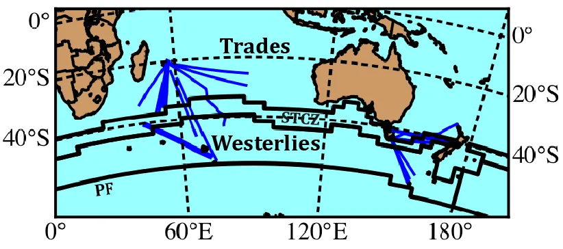
Bio-Acoustic Ships of Opportunity (BASOOP) Program. The data totalled 24 transects 215
covering wide areas of the South West Indian Ocean and Tasman Sea (Fig. 1). Transect 216
length ranged from 200 NM to 1800 NM and included 24hr (day/night) coverage across 217
all seasons between 2009 and 2012. The spatial coverage of the tracks included 2 of the 218
4 major global ocean biomes as described by Longhurst (1998) - the Trades and 219
Westerlies - and also spanned major frontal zones and boundaries including the 220
Subtropical Convergence Zone (STCZ) and the Polar Front (PF). 221
10 225
[FIGURE 1] 226
227
We pre-processed IMOS data by removing dropped pings (a ping is a single acoustic 228
transmit/receive cycle; typical ping rate was 0.5 Hz) and noise spikes (caused for 229
example by violent ship’s motion in rough seas), and partitioned data into separate 230
day/night segments, bounded by sunrise/sunset. In instances where, for example the 231
echosounder had been turned off for short periods, or the vertical sampling resolution 232
of the echosounder was changed, data were further segmented. An acoustic image, or 233
echogram, was created for each segment. The acoustic image was as a two-dimensional 234
array of backscatter values on a depth v time (or space) grid. Each cell in the image, an 235
acoustic pixel, had an associated timestamp, geographical position and depth. For each 236
image, echo intensity in the form of Mean Volume Backscattering Strength (MVBS - 237
Simmonds & MacLennan, 2005) was calculated at a cell resolution of 5m in depth (from 238
the surface down to 1000m) by 1 minute in time. 239
240
2.2 SSL extraction method (SSLEM) 241
242
Our objective was to provide a method that would function over the range of bio-243
acoustical echosounder frequencies in common (and likely future) use, over horizontal 244
scales from bays to oceans, and on vertical scales that encompass microlayers (cm; 245
Holliday et al., 2003) upwards to tens and hundreds of m. The common observational 246
frequency band (18 to 200 kHz) spans the Rayleigh and geometric scattering regions for 247
most zooplankton and nekton. This means that small changes in frequency can result in 248
11 become apparent acoustically when they can be distinguished from background noise 250
(sufficiently high signal-to-noise ratio – SNR). SNR is a function of organism packing 251
density, acoustic Target Strength, depth, insonification frequency and power, and 252
environmental conditions (Simmonds & MacLennan, 2005). SSL appearance may also 253
be influenced by sampling resolution (Korneliussen et al., 2008): for transect data 254
resolution is determined by ping rate, beam angle, depth and ship speed. The 255
geographic scale of data is an important consideration as there are many oceanic 256
processes that occur over different spatial and temporal scales, from micro-turbulence 257
to decadal oscillations. A robust general method should be capable of resolving features 258
of interest at the scale of the study being conducted, and for the organisms of interest in 259
the environment in which they exist. 260
261
2.2.1 Identification of SSLs 262
263
The SSL extraction method (SSLEM) is based upon detection of a contrast in MVBS 264
(Berge et al. 2014) between pixels within SSLs (relatively high MVBS signal) and 265
background pixels outside (relatively low MVBS noise). For a simple SSL analysis, using 266
a window of depth range Z and time/space extent X, one could identify a vertically 267
‘static’ SSL surrounded by empty water by selecting pixels for which MVBS intensities 268
were greater than the mean, µ, over the entire window. Under such a scheme, for any 269
acoustic pixel (px) within the analysis window, 270
Equ. 1 𝑠𝑠𝑙 = {1, 𝑝𝑥 > 𝜇0, 𝑝𝑥 ≤ 𝜇 271
where ssl is a Boolean variable, taking a value of 1 for pixels that are deemed to belong 272
12 the method, assumes that the SSL is completely contained by the analysis window and 274
the surroundings are made up of pixels with low MVBS that is attributable to 275
background noise. This may not be the case; for example, a transition between depth 276
intervals that exhibit a difference in background noise (inherently caused by time-277
varied gain (TVG) amplification of background noise) would yield a layer-like boundary 278
of ssl pixels. To ensure that SSLs were surrounded by lower intensity MVBS (both 279
towards the surface and the seabed), the depth interval of the analysis window was 280
divided into two equal values, d1 and d2, and pixels were only deemed a SSL pixel (ssl
281
value of 1) when their MVBS value was larger than both the MVBS means, µ1 and µ2, 282
over each of the two regions of the split window (Fig. 2a), yielding a new equation for 283
ssl: 284
Equ. 2 𝑠𝑠𝑙 = {1, (𝑝𝑥 > 𝜇1) 𝐴𝑁𝐷 (𝑝𝑥 > 𝜇2)
0, 𝑜𝑡ℎ𝑒𝑟𝑤𝑖𝑠𝑒 285
where µ1 and µ2, are calculated over the regions X by d1 and X by d2 respectively, and 286
where d1 is equal to d2. 287
288
[FIGURE 2] 289
290
In practice, using a fixed analysis window does not capture all SSLs, since they are 291
rarely vertically static: they may for instance oscillate with internal wave activity or 292
migrate vertically. To accommodate this, an analysis column one pixel wide was used 293
instead of a window. The column was moved pixel-by-pixel through the image 294
evaluating the pixel at the centre of the column at each step, such that µ1 and µ2 were 295
calculated over the specific column (single point in time-series), not the entire window, 296
13 values of d1 and d2 this approach would only work if all SSLs had the same thickness and 298
were separated by distances larger than the size of d1 or d2: this is not the case. To 299
overcome this problem the depth ranges d1 and d2, for each pixel evaluated, were varied 300
in size from 2 pixels in height (this minimum, rather than 1, was used to avoid flooding 301
the image with incorrectly assigned ssl pixels when analysing highly variable or ‘noisy’ 302
images) up to the vertical extents of the image (Fig. 2b). Then, for any pixel within an 303
image, evaluated using a dynamic column, 304
305
Equ. 3 𝑠𝑠𝑙 =
{
1, ( ∑ ∑ (𝑝𝑥 > 𝜇1 ) 𝐴𝑁𝐷 (𝑝𝑥 > 𝜇2) 𝑅−𝑟
𝑑2=2 𝑟 − 1
𝑑1=2
) > 0
0, 𝑜𝑡ℎ𝑒𝑟𝑤𝑖𝑠𝑒 306
307
where r is equal to the row number of the pixel being evaluated and R equal to the total 308
number of rows within the image; consequently, the first and last two rows of each 309
image are not processed. Each pixel thus has multiple opportunities (for varying d1 and 310
d2 values) to be attributed an SSL pixel. This ensured that both vertically static and 311
migrant SSLs of varying thicknesses and separation distances would all be identified. 312
313
2.2.2 Phantom SSLs and SSLmin 314
315
On occasions when no SSL was present in the analysis column, pixels would sometimes 316
erroneously be designated as SSL pixels as a result of the backscatter from individual or 317
diffuse arrangements of organisms, tightly packed schools or swarms, variation of the 318
physical properties of sea water, or by natural variation inherent within the data. The 319
14 (measured in space/time units), was therefore introduced to enable the identification of 321
only those SSLs that were relevant to the scale of process being studied e.g. from ocean 322
basin scale (large SSLmin) down to krill swarms (small SSLmin: Watkins et al. 1990). In 323
spite of this precaution, the natural variation within the data still sometimes produced 324
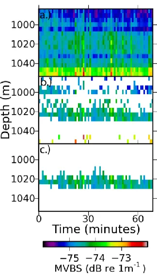
SSLs. These incorrectly identified SSLs, termed ‘phantom SSLs’ (Fig. 3) were removed in 325
post processing (Section 3.1) by analysis of SSL signal-to-noise ratios; SSLs were 326
removed where the mean SSL MVBS (signal) was smaller than the maximum 327
background MVBS value (noise) by analysing the pixels immediately surrounding the 328
layers. 329
330
[FIGURE 3] 331
332
2.2.3 Separation of merged SSLs 333
The SSL pixels identified in Section 2.2.1 were used to generate an SSL mask (Fig. 4b) 334
that bounded pixels that were connected, termed SSL features. These features were not 335
classified as SSLs at this point, as a single feature could consist of several merged SSLs. 336
Features smaller than SSLmin were removed and internal gaps smaller than SSLmin 337
within accepted features were filled (Fig. 4c). 338
339
[FIGURE 4] 340
341
Each feature was then segmented into individual SSLs which existed over a discrete 342
depth range at each point along a time-series. This was achieved by implementing a 343
region-based image segmentation process. A simple growing algorithm moved column 344
15 individual SSLs) within features where SSLs merged or split (Fig. 5). SSLs identified in 346
this process that were smaller than SSLmin were ignored and not analysed further. 347
348
[FIGURE 5] 349
350
2.2.4 Separation of vertically ‘static’ and migrant SSLs 351
352
Vertically static SSLs were separated from upwardly or downwardly-migrating SSLs by 353
application of a Change Point Analysis (CPA: Page 1954). CPA can detect the existence of 354
multiple trends within a time series by analysing the cumulative deviation from the 355
mean over time. The CPA was conducted using a time-series of the mean depth change, 356
ΔZ, over a selected time interval, CPAint, across each SSL (Fig. 6). The choice of CPAint is 357
related to the size of SSLmin. For a relatively large value of SSLmin (> 4 hours for example) 358
a large CPAint value can be chosen and will reduce the likelihood that undulating SSLs, 359
caused by internal waves, would be incorrectly segmented. For small values of SSLmin, a 360
CPAint value should be selected to provide enough samples (>10) for the CPA to be 361
conducted appropriately. The deviation of ΔZ from its mean was calculated (Fig. 6b), 362
followed by the cumulative sum of this deviation (Fig. 6c), the most significant point of 363
change was indicated by the largest absolute value (Fig. 6c – black line), and quantified 364
by the range, CPAmax, of the cumulative sum values. A confidence interval (CI) was 365
calculated by determining the percentage of 1000 bootstrapped samples of ΔZ that 366
yielded a CPAmax value smaller than the original CPAmax value. Where a significant 367
change occurred (95% CI), indicating that a SSL changed from simply varying in depth 368
around a static mean to exhibit migrant behaviour (increasing/decreasing depth), SSLs 369
16 371
[FIGURE 6] 372
373
The CPA was conducted iteratively, until no further statistically significant change (95% 374
CI) within an image segment could be detected: this ensured that multiple migrations, 375
during a diel cycle for example, would all be separated. Multiple migrations were 376
unlikely to occur in this study since at an earlier stage we partitioned the data into 377
separate day and night segments. 378
379
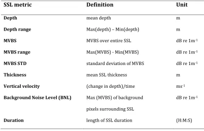
2.2.5 SSL metrics 380
For each individual SSL identified a set of SSL metrics were evaluated (Table 1). The 381
depth, duration, MVBS, MVBS standard deviation, MVBS range and layer thickness 382
described spatial extent and backscatter distribution. The vertical velocity and depth 383
range were used to identify and describe migratory layers. The Background Noise Level 384
(BNL) was used to quantify the maximum level of noise surrounding the SSL. The 385
maximum value was taken to ensure that it would be greater than the mean MVBS value 386
of SSLs consistent of natural variation within the data (phantom SSLs: Section 2.2.2). 387
388
[TABLE 1] 389
390
The SSL metrics were analysed (Section 3.2) to gain better insight into the nature of 391
SSLs within the study region, enabling inferences concerning the pelagic community 392
(spatial arrangement, distribution and heterogeneity) to be made. 393
17 2.3 Validation framework
396
In order to examine the efficacy of our automated SSL identification technique versus 397
the principal present approach, adopted by most acoustic-trawl surveys when assessing 398
fish stocks – visual scrutinisation (which may be subjective and prone to between-399
operator inconsistencies) - we designed a validation framework to examine potential 400
differences between SSLs determined by the SSLEM and visually scrutinised acoustic 401
images. If visual scrutiny gave highly variable results, this would illustrate the difficulty 402
likely to be encountered in comparative studies and the requirement of an automated 403
method. 404
405
The validation was conducted using a subset of the IMOS data. Images from this subset 406
were published online at www.soundscatteringlayers.com. Independent visual scrutiny 407
was performed autonomously by a group of 8 students, all of whom had attended an 408
acoustic data collection and processing summer school 409
(www.depts.washington.edu/fhl/) and were either PhD candidates at the University of 410
St Andrews or the Florida International University. Each student estimated 3 SSL 411
metrics, namely the depth, MVBS and thickness for all SSLs they could identify that 412
persisted for a time period longer than 1 hour. Each student considered 10 images 413
selected randomly from a set of 50. The results of the visual scrutiny were compared to 414
those from SSLEM (see Results 3.1). 415
416
3 Results: 417
Sound Scattering Layers (SSLs) that persisted for time periods longer than 1 hour 418
(SSLmin = 60 minutes; CPAint = 6 minutes: see Sections 2.2.2 and 2.2.4 respectively for 419
18 SSL extraction method (SSLEM). SSLs were extracted at these setting in order to
421
conduct a regional analysis of the study area, ensuring that only persistent and 422
therefore characteristic SSLs were identified. In total, 2064 SSLs were extracted from 423
264 images that were on average 3.4 hours in length; an example of the identification of 424
SSLs for an IMOS image is given in Fig. 4. 108 phantom SSLs (see Section 2.2.2) that 425
were identified in the validation procedure were removed. For each SSL, SSL metrics 426
described in Section 2.2.5 were determined and relationships found between select SSL 427
metrics explored (Section 3.2). 428
429
3.1 SSLEM Validation 430
SSL Metrics that were estimated by the students from SSLs visually identified were 431
mapped back on to the original acoustic images for comparison with the SSLEM 432
identified SSLs. Each visually identified SSL was categorised as being a valid/invalid SSL 433
identification. This process was mirrored using the output from the SSLEM, where 434
phantom SSLs (see Section 2.2.2) were visually identified after extraction and deemed 435
to be invalid SSLs comprised of background noise. The students identified 211 SSLs 436
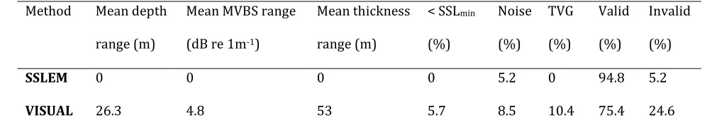
from 80 images. For the same SSLs that were identified by more than 6 of the students 437
from the same image, mean ranges of the estimated metrics were calculated (Table 2). 438
[TABLE 2] 439
440
Of the three SSL identification fields in Table 2 (< SSLmin, Noise & TVG), the Time-441
Varied-Gain (TVG) field contained the largest proportion of the students 442
misclassification of SSLs. The TVG increases the amplitude, as a function of time (or 443
depth for a fixed sound speed) of the echo return and serves to amplify both signal, 444
19 the acoustic image as depth dependent noise (Simmonds & MacLennan, 2005). This 446
essentially limits the useful (range over which signal dominates noise) range of the 447
instrument and causes visible, layer-like bands to form at the far extent of this range. 448
These layers can resemble SSLs to the untrained eye, but not to the SSLEM; normally 449
TVG is removed in pre-processing but can just as easily be removed afterwards (e.g. 450
Watkins & Brierley, 1996). 451
452
The SSLEM identified, on average, over 3 times the number of SSLs per acoustic image 453
than the group of students. Whereas the SSLEM output included no variance between 454
repeat identifications and characterisations of SSLs from the same image, the overall 455
mean standard deviation of the number of SSLs identified per image for the students 456
was 0.54. This is in fact quite low, and demonstrates that although the students 457
identified fewer SSLs, the group broadly did agree on the number of SSLs per image. 458
Metric estimates by the students were, however, notably large, especially the mean 459
MVBS range (4.8 dB re 1m-1) that is equivalent to a factor 3 change in the linear domain. 460
The SSLs identified by the SSLEM were also much more likely to be valid (94.8%), i.e. 461
not phantom SSLs, than those identified by the students (only 75.4% valid), who 462
misidentified SSLs a quarter of the time (Table 2). The SSLEM extracted a total of 108 463
incorrect SSLs, all of which were considered to be phantom SSLs (Section 2.2.2). 464
465
Phantom SSLs form by the naturally occurring variation in the data. They are an artefact 466
of the SSLEM, and hence not detected by visual scrutinisation. This variability is of no 467
consequence within SSLs, but can cause false SSL identification outside (i.e. in empty 468
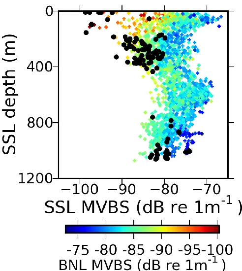
water - Fig. 3). In order to remove phantom SSLs, the Background Noise Level (BNL) 469
20 low BNL-to-MVBS ratios. SSLs that had a MVBS value that was smaller than the BNL 471
were identified as being phantom SSLs (black points in Fig. 7). Removing these SSLs 472
from the results increased the validity of the automated method, for the data analysed 473
in this study, to 100%. 474
475
[FIGURE 7] 476
477
Phantom SSLs are apparent throughout the entire water-column, except for the region 478
between 400m and 800m. In this depth region within the study location of the South 479
West Indian Ocean and Tasman Sea, strong and broad SSLs were persistently present 480
(Fig. 8), meaning that SSLs dominated, excluding the possibility of phantom SSLs 481
forming at the same depth. 482
483
3.2 SSL Metrics 484
The SSLEM output a total of 1956 valid (non-phantom) SSLs from the IMOS data. Each 485
SSL was summarised by a set of 9 SSL metrics (Table 1). 486
487
[FIGURE 8] 488
489
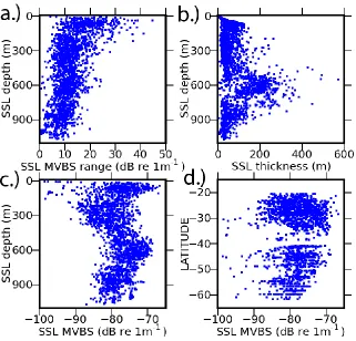
Physical characteristics of SSLs provide biological/ecological insight into pelagic 490
community dynamics. For example, the MVBS range increased towards the surface (Fig. 491
8a) suggesting that the biological community becomes more complex/heterogeneous in 492
the epi-pelagic region; this could be caused by an increase in species diversity or a 493
larger range of the orientations of organisms, caused by feeding for example. The 494
21 column (Fig. 8b). The highest MVBS values (a proxy for increased biomass/abundance) 496
occurred within the water-column at depths of around 600m and at the surface (Fig. 8c) 497
and also geographically towards 40 degrees south (Fig. 8d). This is consistent with the 498
fact that the zone is the highly productive Subtropical convergence zone (see Fig. 1; as 499
identified by Longhurst 1998) where previous work has revealed an enhanced prey-500
field (Boersch-Supan et al. 2012). 501
502
4 Discussion: 503
504
4.1 Sound Scattering Layer Extraction Method (SSLEM) 505
506
The Sound Scattering Layer (SSL) Extraction Method (SSLEM) was demonstrated here 507
using data observed at a single frequency, 38 kHz. However, the method is independent 508
of frequency and is entirely appropriate for use with other frequencies. The main 509
differences that would occur would be subject to the characteristics of the incident 510
frequency, for example, reduced depth range and increased resolution at higher 511
frequencies (Simmonds & MacLennan 2005). 512
513
The efficacy of the SSLEM was examined by comparing output from that of visually 514
scrutinised data (Table 2). The comparison demonstrated that the SSLEM method is 515
more effective at identifying SSLs (Section 3.1). Visually scrutinised images were subject 516
to SSL misclassification, under classification and sample variation, whereas the SSLEM 517
output was perfectly repeatable, with zero variance between repeat extractions of SSLs 518
and metrics. 519
22 Merged vertically static and migrant SSLs were separated by an application of a change-521
point analysis (Section 2.2.4). Analysis of the derived SSL metrics revealed water-522
column and geographical trends (Fig. 8). Summarising these data into discrete metrics 523
offers a method of standardised analysis for assessing variability in biological 524
communities in the water-column. Importantly, acoustic survey data can now be 525
condensed down from millions of values to a set of community descriptors that can be 526
easily stored, shared and analysed. 527
528
4.2 SSLEM Applications 529
530
Analysis of the ocean’s SSLs will enable the study of the ocean’s mid-trophic structure, 531
providing a global prey field that would be invaluable to predator-prey ecologists. SSL 532
depths could be used to gauge energy expenditure of diving mammals (Boersch-Supan 533
et al. 2012; Walters et al. 2014) and spatial arrangements of prey-fields that could be 534
incorporated into existing biophysical models (for example, SEPODYM: Bertignac,
535
Lehodey, & Hampton 1998;Lehodey et al. 1998). Monitoring the structure of SSLs over
536
long time periods could reveal climatic influences and the knock-on effects for SSL 537
inhabitants (Lehodey et al. 2003). Spatially distinct formations of SSLs made up of 538
diverse communities are likely to be distinguished and characterized by SSL metrics, 539
allowing the division of regionally distinct biological communities (Longhurst 1998). 540
Whilst the SSLEM does not resolve communities at the species level, such as the Species 541
Identification Methods from Acoustic Multifrequency Information (SIMFAMI: Gajate et
542
al. 2004) project, the SSLEM offers an alternate and simpler approach for fisheries and
543
conservation management regimes to assess and monitor open ocean ecosystem health 544
23 546
4.3 Summary 547
548
The SSLEM presented here is directly applicable to all acoustic images, including 549
echograms output from Acoustic Doppler Current Profilers (ADCPs), because it is 550
independent of frequency and scale. Furthermore, it naturally lends itself to more 551
complex multi-frequency analysis (Jarvis et al. 2010). Unlike other methods (e.g. Cade 552
and Benoit Bird, 2014), the SSLEM was built to facilitate automated processing of data 553
in a standardised fashion that would vary only with consideration of the resolution and 554
scale of the study in mind. It is our hope that its introduction will enable the analysis of 555
a wealth of data that is immediately available, offering insights into the biological 556
structure of the world’s ocean. The derived SSL metrics provide a means to summarise 557
the extracted layers, making them readily available for a wide range of analysis. 558
Importantly, the SSLEM offers the opportunity to study the structure of the mid-trophic 559
communities in the ocean and will aid in improving our understanding of an ocean 560
ecosystem. 561
562
Acknowledgements:
563
We would like to give special thanks to the reviewers for some very helpful and
564
instructive comments. We would also like to acknowledge the help of the Integrated 565
Marine Observing System data centre (IMOS) and Rick Towler of NOAA for providing 566
vital code for the pre-processing of the acoustic data. Finally we would like to give 567
thanks to the students, namely Katie Kirk, Katie Wurtzell and Laura Hobbs whom 568
attended the Marine Bioacoustics workshop in Friday Harbor, Marta D’Elia from the 569
24 Wiesel from the University of St Andrews, for taking the time to help with the validation 571
of the method. 572
573
Data Accessibility:
574
Acoustic data are publicly available via the Integrated Marine Observing System (IMOS) 575
- Bio-Acoustic Ships of Opportunity (BA SOOP) sub-facility found using the IMOS Ocean 576
data portal: https://imos.aodn.org.au/imos123/home 577
578
References: 579
580
Ainslie, M.A., & McColm, J.G. (1998) A simplified formula for viscous and chemical 581
absorption in seawater. Journal of the Acoustical Society of America, 103, 1671–1672. 582
583
Anderson, C.I.H., Brierley, A.S., & Armstrong, F. (2004) Spatio-temporal variability in the 584
distribution of epi- and meso-pelagic acoustic backscatter in the Irminger Sea, North 585
Atlantic, with implications for predation on Calanus finmarchicus. Marine Biology, 586
146(6), 1177–1188. 587
588
Andreeva, I.B., Galybin, N.N., & Tarasov, L.L. (2000) Vertical structure of the acoustic 589
characteristics of deep scattering layers in the ocean. Acoustical Physics, 46(5), 505–510. 590
591
Brierley, A.S. (2014) Quick Guide: Diel Vetical Migration. Current Biology, 24(22), 1074 - 592
1076. 593
25 Barange, M., Hampton, I., Pillar, S.C., & Soule, M.A. (1994) Determination of composition 595
and vertical structure of fish communities using in situ measurements of acoustic target 596
strength. Canadian Journal of Fisheries and Aquatic Sciences, 51, 99–109. 597
598
Berge, J., Cottier, F., Varpe, Ø., Renaud, P. E., Falk-Petersen, S., Kwasniewski, S., Griffiths,
599
C., Søreide, J.E., Johnsen, G., Aubert, A., Bjaerke, O., Hovinen, J., Jung-Madsen, S., Tveit, M.
600
& Majaneva, S. (2014). Arctic complexity: a case study on diel vertical migration of
601
zooplankton. Journal of plankton research, 36(5), 1279-1297.
602 603
Bertignac, M., Lehodey, P., & Hampton, J. (1998). A spatial population dynamics
604
simulation model of tropical tunas using a habitat index based on environmental
605
parameters. Fisheries Oceanography, 7(3‐4), 326-334.
606 607
Bianchi, D., Stock, C., Galbraith, E.D., & Sarmiento, J.L. (2013) Diel Vertical Migration: 608
Ecological controls and impacts on the biological pump in a one-dimensional ocean 609
model. Global Biogeochemical Cycles, 27, 478-491. 610
611
Bierregaard, R.O., Lovejoy, T.E., Kapos, V., dos Santos, A.A., & Hutchings, R.W. (1992) The 612
biological dynamics of tropical rainforest fragments. BioScience, 42, 859–866. 613
614
Boersch-Supan, P., Boehme, L., Read, J., Rogers, A., & Brierley, A. (2012) Elephant seal 615
foraging dives track prey distribution, not temperature: Comment on McIntyre et al. 616
(2011). Marine Ecology Progress Series, 461(4), 293–298. 617
26 Cade, D.E. & Benoit-Bird, K.J. (2014) An automatic and quantitative approach to the 619
detection and tracking of acoustic scattering layers (supplemental code). Oregon State 620
University Libraries. Software. 621
622
Chapman, R., Bluy, O., Adlington, R., & Robison, A. (1974) Deep scattering layer spectra 623
in the Atlantic and Pacific Oceans and adjacent seas. The Journal of the Acoustical Society
624
of America, 56(6), 1722–1734. 625
626
Coetzee, J. (2000) Use of a shoal analysis and patch estimation system ( SHAPES ) to 627
characterise sardine schools. Aquatic Living Resources, 13(1), 1–10. 628
629
Gajate, J., Ponce, R., Peña, M., Iglesias, M., Fernandes, P., & Alvarez, F. (2004). The
630
SIMFAMI database: a library of ground truthed acoustic survey data. In Annual Science
631
ICES Conference, ICES ASC.
632 633
Godø, O.R., Samuelsen, A., Macaulay, G.J., Patel, R., Hjøllo, S.S., Horne, J., Kaartvedt, S. & 634
Johannessen, J.A. (2012) Mesoscale eddies are oases for higher trophic marine life. PloS
635
One, 7(1), e30161. 636
637
Handegard, N.O., Buisson, L. du, Brehmer, P., Chalmers, S.J., Robertis, A., Huse, G., Kloser, 638
R., Macaulay, G., Maury, O., Ressler, P.H., Stenseth, N.C. & Godø, O.R. (2013) Towards an 639
acoustic-based coupled observation and modelling system for monitoring and 640
predicting ecosystem dynamics of the open ocean. Fish and Fisheries, 14(4), 605-615. 641
27 Hays, G. C. (2003) A review of the adaptive significance and ecosystem consequences of 643
zooplankton diel vertical migrations. Hydrobiologia, 503(1-3), 163–170. 644
645
Holliday, D.V. & Donaghay, P.L., Greenlaw, C.F., Mcgehee, D.E., Mcmanus, M.M., Sullivan, J. 646
M., & Miksis, J.L. (2003) Advances in defining fine- and micro-scale pattern in marine 647
plankton. Aquatic Living Resources, 16, 131–136. 648
649
ICES WGTC: CRR 238 (2000) Editor: Dave Reid, Report on Echo Trace Classification. 650
651
IMOS (2013), IMOS BASOOP sub-facility, imos.org.au [accessed 1st June 2013]. 652
653
Irigoien, X., Klevjer, T. A, Røstad, A., Martinez, U., Boyra, G., Acuña, J. L., Bode, A., 654
Echevarria, F., Gonzalez-Gordillo, J. I., Hernandez-Leon, S., Agusti, S., Aksnes, D. L., 655
Duarte, C. M. & Kaartvedt, S. (2014) Large mesopelagic fishes biomass and trophic 656
efficiency in the open ocean. Nature Communications, 5(May 2013), 3271. 657
658
Jarvis, T., Kelly, N., Kawaguchi, S., van Wijk, E., & Nicol, S. (2010) Acoustic 659
characterisation of the broad-scale distribution and abundance of Antarctic krill 660
(Euphausia superba) off East Antarctica (30-80°E) in January-March 2006. Deep Sea
661
Research Part II: Topical Studies in Oceanography, 57(9-10), 916–933. 662
663
Kawaguchi, S., Nicol, S., Virtue, P., Davenport, S.R., Casper, R., Swadling, K.M. & Hosie, G. 664
W. (2010) Krill demography and large-scale distribution in the Western Indian Ocean 665
sector of the Southern Ocean (CCAMLR Division 58.4.2) in Austral summer of 2006. 666
28 668
Kloser, R.J., Ryan, T.E., Young, J.W. & Lewis, M.E. (2009) Acoustic observations of 669
micronekton fish on the scale of an ocean basin : potential and challenges. ICES Journal
670
of Marine Science, 66, 998–1006. 671
672
Korneliussen, R.J., Diner, N., Ona, E., Berger, L. & Fernandes, P.G. (2008) Proposals for 673
the collection of multifrequency acoustic data. ICES Journal of Marine Science, 65, 982– 674
994. 675
676
Lawson, G. (2001) Species identification of pelagic fish schools on the South African 677
continental shelf using acoustic descriptors and ancillary information. ICES Journal of
678
Marine Science, 58(1), 275–287. 679
680
Lehodey, P., Andre, J. M., Bertignac, M., Hampton, J., Stoens, A., Menkès, C., Memery, L. &
681
Grima, N. (1998). Predicting skipjack tuna forage distributions in the equatorial Pacific
682
using a coupled dynamical bio‐geochemical model. Fisheries Oceanography, 7(3‐4),
317-683
325.
684 685
Lehodey, P., Chai, F., & Hampton, J. (2003). Modelling climate‐related variability of tuna
686
populations from a coupled ocean–biogeochemical‐populations dynamics model.
687
Fisheries Oceanography, 12(4‐5), 483-494.
688 689
Lehodey, P., Murtugudde, R. & Senina, I. (2010) Bridging the gap from ocean models to 690
population dynamics of large marine predators: a model of mid- trophic functional 691
29 693
Longhurst, A. (1998) Ecological Geography of the Sea, Academic Press, San Diego. 694
695
Malhi, Y., Phillips, O.L., Lloyd, J., Baker, T., Wright, J., Almeida, S., Arroyo, L., Frederiksen, 696
T., Grace, J., Higuchi, N., Killeen, T., Laurance, W.F., Leaño, C., Lewis, S., Meir, P., 697
Monteagudo, A., Neill, D., Núñez Vargas, P., Panfil, S.N., Patiño, S., Pitman, N., Quesada, 698
C.A., Rudas-Ll, A., Salomão, R., Saleska, S., Silva, N., Silveira, M., Sombroek, W.G., Valencia, 699
R., Vásquez Martínez, R., Vieira, I.C.G. & Vinceti, B. (2002) An international network to 700
monitor the structure, composition and dynamics of Amazonian forests (RAINFOR). 701
Journal of Vegetation Science, 13(3), 439-450. 702
703
McManus, M.A., Alldredge, A.L., Barnard, A.H., Boss, E., Case, J.F., Cowles, T.J., Donaghay, 704
P.L., Eisner, L.B., Gifford, D.J., Greenlaw, C.F., Herren, C.M., Holliday, D.V., Johnson, D., 705
MacIntyre, S., McGehee, D.M., Osborn, T.R., Perry, M.J., Pieper, R.E., Rines, J.E.B., Smith, 706
D.C., Sullivan, J.M., Talbot, M.K., Twardowski, M.S., Weidemann, A. & Zaneveld, J.R. 707
(2003) Characteristics, distribution and persistence of thin layers over a 48 hour period. 708
Marine Ecology Progress Series, 261, 1–19. 709
710
McManus, M., Cheriton, O., Drake, P., Holliday, D., Storlazzi, C., Donaghay, P. & Greenlaw, 711
C. (2005) Effects of physical processes on structure and transport of thin zooplankton 712
layers in the coastal ocean. Marine Ecology Progress Series, 301, 199–215. 713
714
Nicol, S., Pauly, T., Bindoff, N., Wright, S., Thiele, D., Hosie, G.W., Strutton, P.G. & Woehler, 715
E. (2000) Ocean circulation off east Antarctica affects ecosystem structure and sea-ice 716
30 718
Reid D.G. & Simmonds E.J. (1993) Image analysis techniques for the study of fish school 719
structure from acoustic survey data. Canadian Journal of Fisheries and Aquatic Sciences, 720
50, 886–893. 721
722
Simmonds, E.J. & MacLennan, D.N. (2005) Fisheries Acoustics: Theory and Practice, 2nd 723
edn. Blackwell Publishing, Oxford. 456 pp. 724
725
Stanton, T., Chu, D. & Wiebe, P. (1998) Sound Scattering by several zooplankton groups. 726
II. Scattering models. The Journal of the Acoustical Society of America, 103, 236-253. 727
728
Page, E.S. (1954) Continuous inspection schemes. Biometrika, 100-115.
729 730
Tarasov, L.L. (2002) Deep scattering layers in the northwestern pacific. Acoustical
731
Physics, 48(1), 81–86. 732
733
Walters, A., Lea, M.A., van den Hoff, J., Field, I.C., Virtue, P., Sokolov, S., Pinkerton, M.H. &
734
Hindell, M.A. (2014) Spatially Explicit Estimates of Prey Consumption Reveal a New Krill
735
Predator in the Southern Ocean. PloS one, 9(1), e86452.
736 737
Watkins, J.L., Morris, D.J., Ricketts, C. & Murray, A.W.A. (1990) Sampling biological 738
characteristics of krill: effect of heterogeneous nature of swarms. Marine Biology, 107, 739
409-415. 740
31 Watkins, J.L. & Brierley, A.S. (1996) A post-processing technique to remove background 742
noise from echo integration data. ICES journal of Marine Science, 53, 339-344. 743
744
Wilson, E.O. (1994) Biodiversity: Challenge, science, opportunity. American Zoologist, 745
34, 5–11. 746
32 767
[image:32.595.87.506.111.381.2]768
Table 1 – Sound Scattering Layer (SSL) metrics: summary metrics for individual SSLs. 769
The unit dB re 1m-1 represents 10 times the log base 10 value of a variable with units of 770
m-1, in this case the mean volume backscattering coefficient (Simmonds & MacLennan, 771
2005), that is relative to a reference level of 1m-1. 772
773 774 775 776 777 778 779 780 781
SSL metric Definition Unit
Depth mean depth m
Depth range Max(depth) – Min(depth) m
MVBS MVBS over entire SSL dB re 1m-1
MVBS range Max(MVBS) - Min(MVBS) dB re 1m-1
MVBS STD standard deviation of MVBS dB re 1m-1
Thickness mean SSL thickness m
Vertical velocity (change in depth)/time ms-1
Background Noise Level (BNL) Max (MVBS) of background
pixels surrounding SSL
dB re 1m-1
33 782
Method Mean depth
range (m)
Mean MVBS range
(dB re 1m-1)
Mean thickness
range (m)
< SSLmin
(%)
Noise
(%)
TVG
(%)
Valid
(%)
Invalid
(%)
SSLEM 0 0 0 0 5.2 0 94.8 5.2
VISUAL 26.3 4.8 53 5.7 8.5 10.4 75.4 24.6
[image:33.595.46.548.100.195.2]783
Table 2 – Summary of method output versus visual scrutiny for identification of Sound 784
Scattering Layers (SSLs). Columns definitions from left to right: Method – method of SSL 785
identification; Mean depth range, Mean MVBS range & Mean thickness range – mean 786
ranges of values for the depth, MVBS and thickness metrics for repeat estimations of the 787
same SSLs; < SSLmin – percentage of SSLs identified smaller than the pre-set minimum 788
value; Noise – percentage of SSLs consistent of background noise (including phantom 789
SSLs); TVG – percentage of SSLs made up of ‘layer-like’ noise bands amplified by time-790
varied gain (TVG); Valid – number of correctly identified SSLs; Invalid – number of 791
incorrectly identified SSLs. Percentages and means are to 1 d.p. 792
34 802
Figure 1 - Map showing ship transect lines (blue) for acoustic data extracted from the 803
Integrated Marine Observing System (IMOS) data centre. Mean positions of the 804
Subtropical Convergence Zone (STCZ) and Polar Front (PF) are marked as well as two 805
Longhurst Biomes, the Trades and the Westerlies, separated by the northern boundary 806
of the STCZ. 807
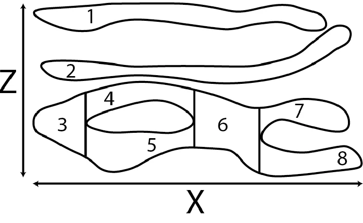
35 819
Figure 2 - Identification of Sound Scattering Layer (SSL) pixels, where green features 820
indicate relatively high intensity SSLs, white background indicates low intensity noise 821
(or empty water) and blue cells represent the SSL pixel being evaluated. a.) Simple SSL 822
analysis window: only vertically static SSLs separated by a distance larger than d1 or d2 823
are detected b.) Dynamic SSL analysis column: a column is moved pixel by pixel through 824
the image, where at each step the column size ranges from the minimum (5 pixels in 825
length; where d1 and d2 are both equal to 2 pixels plus the pixel being evaluated) up to 826
the full vertical extent of the Z axis, by stepping through all the possible values for each 827
of the two parameters, d1 and d2; in doing so, SSLs of varying separation distances and 828
vertical behaviours are captured. 829
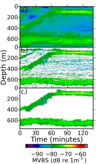
36 835
Figure 3 – Phantom Sound Scattering Layer (SSL) extracted from FV Austral Leader II
836
transect during May 2012, where SSLmin, the minimum horizontal resolution of SSLs, 837
was set to 60 minutes a.) acoustic image segement; b.) SSL pixels identified by the 838
method (Section 2.2.1). c.) Extracted phantom SSL: MVBS values of the SSL are similar 839
to that of the surrounding background. 840
37 849
Figure 4 - Processed acoustic image, from FV Austral Leader II transect during May 850
2012, where SSLmin, the minimum horizontal resolution of Sound Scattering Layers 851
(SSLs), was set to 60 minutes. a.) Original acoustic image at a resolution of 5m in depth 852
and 1 minute in time. b.) Masked image: only pixels that are deemed to be potential SSL 853
pixels are shown. c.) SSLs identified after removing features smaller than SSLmin and 854
filling SSL internal gaps (that are smaller than SSLmin). 855
38 864
Figure 5 - Segmentation of Sound Scattering Layers (SSLs) features into 865
individual SSLs. Each SSL was assigned a unique index value. 866
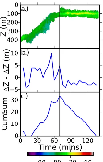
39 880
Figure 6 - Change Point Analysis of mean Sound Scattering Layer (SSL) depth – SSL 881
taken from the example image in Fig. 4. The vertical black line at 70 minutes - the 882
maximum point of the cumulative sum of b.) - indicates the point of separation of a 883
static SSL and a migrant SSL. a.) SSL depth b.) The overall mean depth change of SSL 884
minus each mean depth change in the time-series (binned at 6 min intervals) plotted in 885
time c.) Cumulative sum of b: the maximum value indicates the most significant point of 886
change. 887
40 895
Figure 7 – Background Noise Level (BNL) for Sound Scattering Layers (SSLs) extracted 896
from the IMOS dataset by SSL depth and MVBS. Black points represent phantom SSLs 897
(incorrectly assigned SSLs) identified where BNL > SSL MVBS. 898
41 910
Figure 8 – Sound Scattering Layer (SSL) metrics extracted from the IMOS dataset. a.) 911
Water column heterogeneity: MVBS range serves as a proxy for biological complexity; 912
b.) SSL thickness as a function of depth; c.) Depth distribution of MVBS; d.) Latitudinal 913
distribution of MVBS. 914