3313
INTRODUCTION
When an insect hovers, the centre of mass of its body oscillates around a point in the air and its body angle (pitch angle) oscillates around a mean value, because of the periodically varying aerodynamic and inertial forces of the flapping wings. Similar oscillations exist in other flight modes (e.g. forward flight). In previous experimental and computational fluid dynamics (CFD) studies on insect aerodynamics [e.g. experimental studies (Ellington et al., 1996; Dickinson et al., 1999; Sane and Dickinson, 2001; Usherwood and Ellington, 2002a; Usherwood and Ellington, 2002b); CFD studies (Liu and Kawachi, 1998; Wang, 2000; Ramamurti and Sandberg, 2002; Sun and Tang, 2002a; Sun and Tang, 2002b)], the body dynamics was not included and the oscillations of the body centre of mass and body angle were neglected (the body was assumed to be fixed at a point or to move at a constant velocity). For insects with a relatively high wingbeat frequency and a small ratio of wing mass to body mass, the oscillations of the body would be very small and could be neglected. But for insects with a relatively low wingbeat frequency and a large ratio of wing mass to body mass, how large would be the effect of the body oscillations on the aerodynamic forces and moments? Moreover, in the study of flight dynamics (dynamic stability and control) of insects, the ‘equilibrium flight’ must be
given first. With body oscillations, the state variables at equilibrium flight are periodical functions of time. These periodical functions must be obtained before stability and control analysis can be conducted. As a result, it is of great interest to obtain the periodical solutions of the body motion at equilibrium flight.
In the present study, we couple the equations of motion with the fluid flow equations (the Navier–Stokes equations) to simulate the hovering (including body oscillations) of some model insects, obtaining the periodical solutions of the equilibrium flight. The results can tell us how body oscillations affect the aerodynamic forces and moments. Moreover, the results can provide the periodical solutions of equilibrium flight, based on which the flight stability and control problems can be studied.
Two model insects are considered. One is a model dronefly and the other a model hawkmoth. The model dronefly may represent insects with a relatively high wingbeat frequency and a small wing mass to body mass ratio; the model hawkmoth may represent insects with a relatively low wingbeat frequency and a large wing mass to body mass ratio (for the dronefly, the wingbeat frequency is about 160 Hz and the wing mass to body mass ratio is about 1%; for the hawkmoth, the corresponding values are 26 Hz and 6%). Another reason for choosing these insects is that their morphological and wing kinematic data at hovering are available.
The Journal of Experimental Biology 212, 3313-3329 Published by The Company of Biologists 2009 doi:10.1242/jeb.030494
Hovering of model insects: simulation by coupling equations of motion with
Navier–Stokes equations
Jiang Hao Wu
1, Yan Lai Zhang
2and Mao Sun
2,*
1School of Transportation Science and Engineering and2Ministry of Education Key Laboratory of Fluid Mechanics, Institute of Fluid
Mechanics, Beijing University of Aeronautics and Astronautics, Beijing, China
*Author for correspondence ([email protected])
Accepted 1 July 2009
SUMMARY
When an insect hovers, the centre of mass of its body oscillates around a point in the air and its body angle oscillates around a mean value, because of the periodically varying aerodynamic and inertial forces of the flapping wings. In the present paper, hover flight including body oscillations is simulated by coupling the equations of motion with the Navier–Stokes equations. The equations are solved numerically; periodical solutions representing the hover flight are obtained by the shooting method. Two model insects are considered, a dronefly and a hawkmoth; the former has relatively high wingbeat frequency (n) and small wing mass to body mass ratio, whilst the latter has relatively low wingbeat frequency and large wing mass to body mass ratio. The main results are as follows. (i) The body mainly has a horizontal oscillation; oscillation in the vertical direction is about 1/6 of that in the horizontal direction and oscillation in pitch angle is relatively small. (ii) For the hawkmoth, the peak-to-peak values of the horizontal velocity, displacement and pitch angle are 0.11U (U is the mean velocity at the radius of gyration of the wing), 0.22c=4 mm (c is the mean chord length) and 4 deg., respectively. For the dronefly, the corresponding values are 0.02U, 0.05c=0.15 mm and 0.3 deg., much smaller than those of the hawkmoth. (iii) The horizontal motion of the body decreases the relative velocity of the wings by a small amount. As a result, a larger angle of attack of the wing, and hence a larger drag to lift ratio or larger aerodynamic power, is required for hovering, compared with the case of neglecting body oscillations. For the hawkmoth, the angle of attack is about 3.5 deg. larger and the specific power about 9% larger than that in the case of neglecting the body oscillations; for the dronefly, the corresponding values are 0.7 deg. and 2%. (iv) The horizontal oscillation of the body consists of two parts; one (due to wing aerodynamic force) is proportional to 1/cn2
and the other (due to wing inertial force) is proportional to wing mass to body mass ratio. For many insects, the values of 1/cn2and wing mass to body mass ratio are much
smaller than those of the hawkmoth, and the effects of body oscillation would be rather small; thus it is reasonable to neglect the body oscillations in studying their aerodynamics.
3314
MATERIALS AND METHODS Equations of motion of an insect
Equations of motion for a model insect with a body and a number of flapping rigid wings have been derived by Sun and colleagues (Sun et al., 2007). Three frames of reference are used in the derivation (Fig. 1): frame (xE,yE,zE) is an inertial frame (a frame fixed
on the earth);xEis in the horizontal direction and zEin the vertical
direction. Frame (xb,yb,zb) is a frame fixed on the insect body with
its origin at the centre of mass of the wingless body;xb, yband zb
are the longitudinal, transverse and dorsoventral body axes, respectively. Frame (xw,yw,zw) is a frame fixed on an insect wing
with its origin at the root of the wing; xwis in the spanwise direction,
pointing to the wing tip, and zwis in the chordwise direction, pointing
to the trailing edge of the wing. With respect to the inertial frame, the centre of mass of the wingless body moves at velocity νcg, the
body rotates at angular velocity ωbd(angular velocity of the wing
relative to the body is prescribed). The equations of motion can be written as (see Appendix A):
wherebνcgand bωbdrepresent the xb, yband zbcomponents of νcg
and ωbd, respectively; and Frepresents the inertial, aerodynamic
and gravitational forces and moments of the body and wings (see Appendix A).
Some terms in the right-hand side of Eqn 1 are dependent on the orientation of the insect body, and the equations that govern the Euler angle rates of the body are needed. For longitudinal motion, the differential equation of the body pitch angle is:
where θbis the pitch angle of the body (angle between xband the
horizontal) and qbis the pitch rate, i.e. the ybcomponent of ωbd.
The system of equations, Eqns 4 and 5, is integrated using a modified Euler method. The aerodynamic force and moment terms in Eqn 1 must be obtained by solving the fluid flow equations, i.e. the Navier–Stokes equations (see below for a description of how the equations of motion are coupled with the Navier–Stokes equations in the solution process).
Fluid dynamics equations
The aerodynamic forces and moments in Eqn 1 are determined by the Navier–Stokes equations:
where uis the fluid velocity,pthe pressure,ρthe density, νthe kinematic viscosity, =the gradient operator and =2the Laplacian
operator.
To obtain the aerodynamic forces and moments, in principle we need to compute the flows around the wings and the body. But near hovering, the aerodynamic forces and moments of the body are negligibly small compared with those of the wings because the velocity of the body is very small. Therefore, we only need to compute the flows around the wings. We further assume that the contralateral wings do not interact aerodynamically and neither do the body and the wings. Sun and Yu showed that the left and right wings had negligible interaction except during ‘clap and fling’
ν
·
∂u
∂t +u ∇u= −
1
ρ ∇p+ ν∇
2u , (3b)
ν
∇· u=0 , (3a)
ν
dθb
dt =qb, (2)
d dt
bνcg bbd
⎡
⎣ ⎢ ⎢
⎤
⎦ ⎥
⎥=F, (1)
motion (Sun and Yu, 2006); Aono and colleagues showed that the interaction between wing and body was negligibly small: the aerodynamic force of the case with the body–wing interaction differs by less than 2% from that without body–wing interaction (Aono et al., 2008). Therefore, the above assumptions are reasonable. Thus in the present flow computation, the body is neglected and the flows around the left and right wings are computed separately.
The computational methods used to solve the Navier–Stokes equations are the same as those described by Sun and Tang (Sun and Tang, 2002a). The algorithm was based on the method of artificial compressibility. The computational grid has dimensions 93⫻109⫻78 in the normal direction, around the wing section and in the spanwise direction, respectively; the normal grid spacing at the wall was 0.0015 (portions of the grids are shown in Fig. 2). The outer boundary was set at 20 chord lengths from the wing. The non-dimensional time step was 0.02 (non-non-dimensionalized by c/Uwhere
c is the mean chord of the wing of the insect and U is the mean flapping speed of the wing; see below for the definition of U). A detailed study of the numerical variables such as grid size, domain size, time step, etc., was conducted and it was shown that the above values for the numerical variables were appropriate for the calculations. Boundary conditions are as follows. For the far-field boundary condition, at the inflow boundary, the velocity components are specified as free-stream conditions (determined by flight speed), whereas pressure is extrapolated from the interior; at the outflow boundary, pressure is set equal to the free-stream static pressure and the velocity is extrapolated from the interior. On the wing surfaces, impermeable wall and non-slip conditions are applied and the pressure is obtained through the normal component of the momentum equation written in the moving grid system.
J. H. Wu, Y. L. Zhang and M. Sun
Fig. 1. Reference frames. (xE,yE,zE), frame fixed on the earth; (xb,yb,zb),
frame fixed on the insect body with its origin at the centre of mass of the body, xb-axis along the long-axis of the body and ybin the right side
direction; (xw,yw,zw), frame fixed on the wing, with its origin at the wing root,
xw-axis along the wing span and zw-axis along the chordwise direction. Rcg,
vector of the centre of mass of the body relative to the earth frame; Rh,
3315 Hovering of model insects
The integration method of coupling the equations of motion with the Navier–Stokes equations
The equations of motion (Eqns 1 and 2) and the Navier–Stokes equations (Eqn 3) must be coupled in the solution process because the aerodynamic forces and moments in the equations of motion must be obtained from the solution of the Navier–Stokes equations and the boundary condition of the Navier–Stokes equations must be obtained from the motion of the insect determined by the equations of motion. Let uband wbdenote the xband zbcomponents
of b–νcg, respectively, and qbdenote the ybcomponent of bcg(note
that in hovering, flight is symmetrical about the longitudinal plane and other components of ν–cg and ωbd are zero). The integration
process is as follows. Suppose that at time tnthe motion of the insect body (ub, wb, qband θb) are known (the wing motion with respect
to the body is prescribed), the boundary condition of the Navier–Stokes equations would be known and the flow equations can be solved to provide the aerodynamic forces and moments at this time station; then Eqns 1 and 2 are marched to the next time station tn+1, using the Euler predictor-corrector method; the process
is repeated in the next step, and so on (see below for how the calculation starts). The Euler predictor-corrector method is described below.
Let x represent the vector of unknown variables of the body motion, or the state variables [ubwbqb]Tand f(x,t) represent the
vector function on the right side of the system of Eqns 1 and 2. The equations of motion can be written as:
The Euler predictor-corrector method has two steps (e.g. Gerald, 1978). First step, estimating (predicting) the value of xattn+1using
the single Euler method (let x*n+1denote the estimated value):
ν
x*n+1=xn+
(
tn+1−tn)
·f x(
n,tn)
. (5) νdx
dt = f(x,t) . (4)
Second step, obtaining the corrected value of xattn+1:
The time accuracy of the integration method is of second order.
The method of finding the periodic solution
As mentioned above, in the flight of an insect, because of the cyclic force and moment of the flapping wings, the velocity of the centre of mass and the pitch angle of the body oscillate around some mean values. For hovering flight, the mean velocity and mean pitch rate are zero, and the mean pitch angle is a constant. Therefore, we are looking for periodic solutions of Eqns 1 and 2 with zero mean horizontal and vertical velocities and pitch rate. If the periodic solutions were stable, a forward integration of the equations would converge to the solutions. But linear stability analysis showed that hovering and forward flight were unstable (Taylor and Thomas, 2003; Sun and Xiong, 2005; Sun et al., 2007). Therefore, in the present study, the shooting method is used to find the periodical solutions. This method is described by Ling (Ling, 1983) (see also Fehlberg, 1969). In the shooting method, the initial conditions are iterated, so that they coincide with the terminal conditions. The method is outlined here and a detailed description is given in Appendix B. The equations of motion (Eqn 4) and the periodical conditions are:
where Tis the period of the solution (in the present study, Tis known and is the wingbeat period). A vector parameter,s, is introduced, and it is chosen as x(0). Eqn 7 can be written as:
where g(s) is a vector function representing the dependence of the equations ons; x(0; s)=s.sis iterated using Newton’s method until the boundary conditions, i.e. F(s)=0, are satisfied to an acceptable accuracy (see Appendix B for the detailed procedure).
How the calculation starts and the solution process In the shooting method described in the preceding section and Appendix B, the equations of motion are repeatedly integrated from
t=0 to t=Twith different initial conditions (initial state variables of the insect’s body, ub, wb, qband θb), until the state variables at t=0
are equal to those at t=T. During each of the iterations, the Navier–Stokes equations need to be solved only in one wingbeat period (from t=0 to t=T). Note that flow is unsteady and the solution of unsteady Navier–Stokes in the period from t=0 to t=Tdepends on the flow field before t=0; specifically, on the flow field at the time step before t=0 (i.e. at t=–Δt; Δt is the time step). Since the flow is periodical in time, the flow field at t=–Δt is the same as that at t=T–Δt. But the flow field at t=T–Δt is not known until the equations of motion and the Navier–Stokes equations are solved in the period fromt=0 to t=T.
How, then, can we obtain the flow field at t=–Δt? Let us look at the flow problem in which the model insect starts to beat its wings at t=0 (the first downstroke is from t=0 to t=0.5T) without body motion (see next section for the description of the wing motion). At t=0, the flow velocity is zero everywhere. With the known flow
ν
.
xn+1= xn+
(
tn+1−tn)
·⎡⎣f x(
n, tn)
+ f x(
*n+1, tn+1)
⎤⎦ 2 (6)ν
dx
dt = f(x,t) , (7a)
ν
x(0)−x(T)=0 , (7b)
ν
F(s)= x(0;s)−x(T;s)=0 , (8b)
ν
dx
dt = f[(x,t;g(s)] , (8a) xw
xw
A
B
3316
field at t=0, the Navier–Stokes equations are solved to give flows and aerodynamic forces at later times. Fig. 3 shows the computed lift, drag and pitching moment coefficients of the wing (denoted by
CL, CDand CM, respectively; see below for the definitions of the
coefficients). In the first half-stroke (t=0 to t=0.5T), the aerodynamic forces are relatively large (this is because there is no previous wake to produce the induced effects). After less than three cycles, the forces and moment become approximately periodic. Usherwood and Ellington (experiment with revolving wings), Ramamurti and Sandberg (CFD computation of 3-dimensional flapping wings), and Wang (CFD computation of 2-dimensional wing) also reported that after the start of the wingbeat, the forces became periodic in less than three cycles (Usherwood and Ellington, 2002a; Ramamurti and Sandberg, 2002; Wang et al., 2004). This shows that the periodic wake of a flapping wing is established in less than three cycles after the wing starts to beat.
If the body of the insect oscillates, the established periodic wake of the flapping wing would be different from that in the above case of a fixed body. But if the velocity of the body oscillation is much smaller than that of the tip speed of the flapping wing, the difference in the established wake between these two cases would be small. This is because when the body velocity is much smaller than the speed of wing flapping, the wing flapping would dominate the wake production. Thus, when the body oscillation is small, we could use the established wake of the case without body oscillation to approximate that of the case with body oscillation. Let us test this
by the following two flow computations. In the first one (caseα), the body oscillates in the horizontal direction sinusoidally for four cycles (t=0 tot=4T); the amplitude of the horizontal velocity is 0.06U (where Uis the mean flapping velocity of the wing, see below for its definition). In the second computation (case β), from t=0 to
t=3T–εT (where εis a small number, here ε=0.1), the body is fixed; from t=3T–εTto t=3T, the body velocity changes smoothly from zero to that of caseαat t=3T; fromt=3Tto t=4T, the body motion is the same as that of case α(see Fig. 4A,B). In both cases, the flapping motion of the wing is the same. Note that in the fourth cycle (t=3Tto t=4T), both the wing flapping motion and the body motion are the same for the two cases. Fig. 4C compares the computed CLvalues in the fourth cycle of the two cases; they are
almost identical (the same is true for the computed CDand CM, not
shown here; in the above computation, ε is 0.1; we tried with ε varying between 0.05 and 0.2 and no difference was observed in the results of the fourth period). This shows that replacing the wake generated in the first three cycles by the flapping wing of the case with a small body oscillation (case α) with that of the case without
J. H. Wu, Y. L. Zhang and M. Sun
CL
CD
CM
0 1 2 3 4 5 6 7
0 2
4
A
0 1 2 3 4 5 6 7
–2 0 2
B
0 1 2 3 4 5 6 7
–4 –2 0 2
4
C
t/T
Fig. 3. Time courses of the lift (CL), drag (CD) and moment (CM) coefficients
of a wing of the model dronefly (body fixed). t, time; T, wingbeat period.
x
. e,b
/
U 0 1 2 3 4
–0.1 0 0.1
A
0 1 2 3 4
–0.1 0 0.1
B
3 3.2 3.4 3.6 3.8 4
–1 0 1 2
3
4
Case α Case β Case α
Case β
C
CL
t/T
Fig. 4. (A,B) Time courses of the horizontal velocity of the body centre of mass in four cycles, of case αand case β, respectively. (C) Comparison of the lift coefficient in the fourth cycle between case αand case β. xE,b/U,
non-dimensional horizontal velocity of centre of mass; CL, lift coefficient; t,
3317 Hovering of model insects
body oscillation (case β) has negligible effect on the later flow computation.
Now, let us go back to the question raised above: in the calculation of coupling the equations of motion with the Navier–Stokes equations, the calculation is carried out in one period,
t=0 to t=T; how is the flow field att<0 given? On the basis of the above discussion, we assume that when the body oscillations are small, one can use the flow field established by the insect without body oscillation to provide the required initial flow field data.
With the above assumption, the solution process for obtaining the periodic solutions is as follows:
1. Guess the initial values of the state variables of the body, i.e. ub, wb, qb and θbatt=0. In the first iteration, we set them as: ub=0, wb=0, qb=0 and θb=χ(where χis the mean body angle, known from
measured data). It should be noted that in the later iterations, generally, the initial values of ub, wbandqbwould not be zero and
that of θbwould not be χ. For convenience, we write the initial
values as s1, s2, s3and s4.
2. Start the wingbeat at t=–3T, with the body fixed (ub, wb, qb=0
and θb=χ), and at the same time start to compute the flow with the
Navier–Stokes equations. Fromt=–0.1Ttot=0, ub, wb, qband θb
change smoothly from zero to their initial values, s1, s2, s3and s4,
respectively.
3. At t=0, start the computation of coupling the equations of motion and the Navier–Stokes equations (the flow field at the time step before t=0, which is needed for solving the Navier–Stokes equations at t≥0, is provided by the flow solution in step 2), and obtain the solution in the period from t=0 to t=T.
4. Compare the values of ub, wb, qband θbatt=Twith those at t=0,
i.e. s1, s2, s3and s4. If they are respectively equal, the periodic solution
is obtained and the calculation finished. If not, go to the next step. 5. This step includes six ‘sub-steps’ to obtain the Jacobian matrix in Newton’s method (see Appendix B) and the new initial values. (i) Change the initial value of ubby a small quantity, Δs1, and obtain
a set of sub-step initial values: s1+ Δs1,s2, s3and s4. Using the set
of initial values, conduct the computation in steps 2 and 3 and obtain
F(s*,1).
(ii) Change the initial values of wbby Δs2and obtain a second set
of sub-step initial values: s1, s2+ Δs2,s3 and s4. Similarly, obtain F(s*,2).
(iii) Similarly, obtain F(s*,3). (iv) Similarly, obtain F(s*,4).
(v) Compute the Jacobian matrix.
(vi) Using the Jacobian matrix, compute the new initial values. With the new initial values, go to step 2 for the next iteration.
The wings, the flapping motion and the morphological and flight data
The model wings used in the present study are flat plates with rounded leading edges; the thickness is 3% of the mean chord length. The platforms of the model wings of the dronefly and the hawkmoth are obtained from the measured data of Liu and Sun, and Ellington (Liu and Sun, 2008; Ellington, 1984a), respectively (Fig. 2). The
flapping motion of a wing is assumed as follows. The motion consists of two parts: the translation (azimuthal rotation) and the rotation (flip rotation); the out-of-plane motion of the wing (deviation) is neglected. The time variation of the positional angle (φ) of the wing is approximated by the simple harmonic function:
where nis the wingbeat frequency, θthe mean stroke angle and Φ the stroke amplitude. The angle of attack of the wing (α) takes a constant value during the downstroke or upstroke translation (the constant value is denoted by αdfor the downstroke translation and
αufor the upstroke translation); around stroke reversal, the wing
flips and α changes with time, also according to the simple harmonic function. The function representing the time variation of αduring the supination at themth cycle is:
where Δtris the time duration of wing rotation during the stroke
reversal and ais a constant:
t1is the time when the wing rotation starts:
The expression of the pronation can be written in the same way. For the dronefly, Eqns 9 and 10 are good approximations to the measured data (Liu and Sun, 2008; Ellington, 1984b); whilst for the hawkmoth, φ(t) is a little different from the simple harmonic function (Willmott and Ellington, 1997a; Willmott and Ellington, 1997b). From Eqns 9 and 10, we see that to prescribe the flapping motion, the stroke amplitude Φ, the wingbeat frequency n, the time duration of wing rotation Δtr, the angles of attack in the downstroke
and upstroke translations αdand αu, and the mean positional angle
φmust be given.
Morphological and wing motion parameters for the dronefly are taken from the data of Liu and Sun (Liu and Sun, 2008) and that for the hawkmoth from the data of Willmott and Ellington (Willmott and Ellington, 1997a; Willmott and Ellington, 1997b). It should be noted that moments and products of inertia of the wing are not given in these references and they are estimated using the data of Liu and Sun, Willmott and Ellington, and Ennos (Liu and Sun, 2008; Willmott and Ellington, 1997a; Willmott and Ellington, 1997b), according to the density distribution of a dronefly wing measured by Ennos (Ennos, 1989b).
The morphological data for the wings are listed in Table 1: mwg
is the mass of one wing; Ris wing length; c is the mean chord length of the wing; Sis the area of one wing; r2, is the radius of
the second moment of wing area; Ix,w, Iy,wand Iz,ware moments of
inertia of the wing about the xw, ywand zwaxes, respectively; and Ixy,wis the product of inertia of the wing.
The morphological data for the bodies are listed in Table 2: mb
is the mass of the body; Iy,bis the moment of inertia of the body
ν
φ = φ +0.5Φcos(2πnt) , (9)
ν
α = αd+a{(t−t1)−Δt r
2πsin[2π(t−t1) /] Δtr}, t1≤t≤t1+ Δtr , (10a)
ν
t1=mT−0.5T− Δtr/ 2 . (10c) ν
[image:5.612.49.568.674.721.2]a=(180π − αu− αd) /Δtr ; (10b)
Table 1. Morphological data of wing
mwg R c S Ix,w Iy,w Iz,w Ixz,w
ID (mg) (mm) (mm) (mm2) r
2/R (kg m2) (kg m2) (kg m2) (kg m2)
DF 0.56 11.2 2.98 33.34 0.55 5.23⫻10–13 1.25⫻10–11 1.20⫻10–11 8.04⫻10–13
HM 46.82 48.5 18.37 890.9 0.51 1.59⫻10–9 1.94⫻10–8 1.78⫻10–8 3.86⫻10–10
DF, model dronefly; HM, model hawkmoth; mwg, mass of one wing; R, wing length; c, mean chord length of wing; S, area of one wing; r2, radius of second
3318
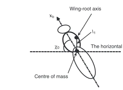
about the yb-axis;lbis body length; l1is the distance between the
wing-base axis and the centre of mass of the body; and χ0is the
free body angle [the definitions of χ0and l1 are given in Fig. 5,
following Ellington (Ellington, 1984a)]. For longitudinal motion, the body morphological parameters needed in equations of motion are the body mass, moment of inertia, and the relative position of the wing-base axis and the centre of mass. Withχ0and l1known,
the relative position of the wing-base axis and the centre of mass of the body can be determined. In the papers by Ellington and by Liu and Sun, the centre of mass (or values of χ0 and l1) was
determined as follows: two pictures showing the lateral and dorsoventral views of the body were taken; the cross-section of the body was taken as an ellipse and a uniform density was assumed, and then the position of the centre of mass can be computed (see Ellington, 1984a).
The wing and body kinematic data are listed in Table 3: Φis the stroke amplitude; nis the wingbeat frequency; Δtris the wing rotation
time; βis the stroke plane angle; χis the mean body angle; Re, is the the Reynolds number of a wing (the mean flapping velocity, U, is defined as U=2Φnr2and the Reynolds number of a wing is defined
as Re=cU/νwhere νis the kinematic viscosity of the air). From Tables 1–3, we see that all needed morphological and wing-kinematic parameters have been given, except αd, αuand. These
three parameters are difficult to measure accurately and they will be obtained during the solution process, using the condition of equilibrium flight (see below).
RESULTS
Test of the equations of motion and the computation codes The code used for the flow computation was tested by Wu and Sun (Wu and Sun, 2004) using experimental data of flapping and rotating model insect wings; and recently, it was further tested by Sun and
Yu (Sun and Yu, 2006) using experimental data for a flinging wing pair.
Here, we test the correctness of the equations of motion and their solution code by the following approach. Suppose that the model insect flaps its wings in the vacuum space without gravity; then an analytical solution of the problem exists, i.e. the centre of the total mass of the insect remains at the same point in space. Fig. 6 shows the time histories of the horizontal velocity of the centre of the total mass, together with that of the centre of the body mass, for the model dronefly which beats its wings in a horizontal plane with αd=αu=90 deg., =0, Φ=107 deg. and n=164 Hz (the vertical velocity
of the centre of the total mass and that of the centre of the body mass are both zero and are not shown here; the calculation was carried up to a time of 300 wingbeats, but only results in the first 30 cycles are shown here). It can be seen that the centre of the total mass remains motionless; the centre of the body mass has a horizontal oscillation, because the wings oscillate in a horizontal plane. Integrations using various time step values showed that when the non-dimensional time step value (non-dimensionalized by c/U) was 0.02 (about 400 time steps in one cycle), the results changed by less than 0.02% when the time step was further halved.
Obtaining the periodical solutions of hover flight If all the wing motion parameters are known, the periodical solutions of the hover flight can be solved directly using the methods given in Materials and methods. But as aforementioned, the downstroke and upstroke angles of attack (αdandαu) and the mean stroke angle
() of the wings are not known; they are to be determined by the hover flight conditions: the mean vertical and horizontal velocities of the centre of mass of the body are zero and the mean pitch angle of the body is a constant (or the mean vertical aerodynamic force of the wings balances the weight of the insect and the mean
[image:6.612.44.296.80.129.2]J. H. Wu, Y. L. Zhang and M. Sun
Table 2. Morphological data for body
mb lb χ0 Iy,b
ID (mg) (mm) l1/lb (deg.) (kg m2)
DF 87.76 14.11 0.13 52 1.18⫻10–9
HM 1485 42.49 0.26 82.9 1.42⫻10–7
DF, model dronefly; HM, model hawkmoth; mb, mass of body; lb, body
length; l1, distance between the wing-base axis and the centre of mass of
the body; χ0, free body angle; Iy,b, moment of inertia of body about yb-axis.
Wing-root axis
xb
χ0
l1
Centre of mass
The horizontal
Fig. 5. The definitions of free body angle (χ0) and the distance between the
wing-root axis and body centre of mass (l0). xb, an axis of the body frame
(see Fig. 1).
0 5 10 15 20 25 30
–0.04 0 0.04
x
. E,t
/
U,
x
. E,b
/
U
x.E,t/U x .
E,b/U
t/T
Fig. 6. The time histories of the horizontal velocity of the total centre of mass (xE,t) and that of the body centre of mass (xE,b) of the model dronefly.
[image:6.612.48.247.564.709.2]U, mean flapping velocity; T, wingbeat period; t, time.
Table 3. Kinematic data of wing and body
Φ n β χ
ID (deg.) (Hz) Δtr/T (deg.) (deg.) Re
DF 107.1 164 0.3 0 42 782
HM 114.4 26.1 0.3 0 54.8 3315
DF, model dronefly; HM, model hawkmoth;Φ, stroke amplitude; n, wingbeat frequency; Δtr, wing rotation time; T, wingbeat period; β, stroke plane
[image:6.612.330.561.565.712.2]3319 Hovering of model insects
horizontal aerodynamic force and the aerodynamic pitch moment around the centre of mass of the body are zero).
We determine the values of αd, αu and and the periodical
solutions of the hovering insects in the following two steps.
Step 1: αd, αuand in the case of no body oscillations In our previous work on the hovering flight of insects (e.g. Sun and Tang, 2002b; Sun and Du, 2003), the body was assumed to be fixed in the air and αd, αuand were determined by the force and moment
equilibrium conditions: a set of values of αd, αuand were guessed;
the flow equations were solved and the mean vertical force (Ze),
mean horizontal force (Xe) and mean pitch moment (Me) were
calculated; if the magnitude of Zewas not equal to the weight, or Xeor Me was not equal to zero, αd, αuand were adjusted; the
calculations were repeated until the magnitude of Ze was
approximately equal to the weight, and Xe and Me were
approximately equal to zero. Experimental observations showed that for many insects, αdandαuwere about 35 deg. and was not far
from zero (Ellington, 1984b). These values were used as the starting values in the computations. Using starting values of αd, αuand
that were not far from the real values can reduce the number of repeated computations; more importantly, there could be more than one set of αd, αuand satisfying the equilibrium conditions due
to the non-linearity in the aerodynamic force production, and by so doing, the calculation could generally converge to the realistic solution. Since body oscillation was not considered, values of αd,
αuand determined in this way must be different from those when
the body is free to oscillate. But it is expected that the difference would not be very large. As will be seen below, αd, αuand values
determined in this way are useful in determining the αd, αuand
values when the body is free to oscillate.
Using the above method, we found that without body oscillations, for the dronefly, when αd=αu=31.8 deg. and =2.8 deg., the mean
vertical force of the wings approximately balanced the weight, and the horizontal force and pitch moment are approximately zero. For the hawkmoth, the corresponding values are αd=38.3 deg.,
αu=39.5 deg. and =11 deg.
Step 2: solutions with body oscillations
The αd, αuand values obtained above give forces and moments
satisfying the equilibrium conditions in the case of a body held fixed. When the body is free to oscillate, these αd, αuand values would
not give the correct forces and moments for hovering. But it is expected that these αd, αuand values are not too far from the
correct ones, and that when these values are used, the insect would have a near-hovering flight, i.e. would fly at a very small velocity. Based on the flight speed and direction, we can adjust the values of αd, αuand until an approximate hovering flight, i.e. with mean
horizontal and vertical velocities and mean pitch rate being approximately zero, is obtained. Note that the horizontal and vertical velocities of the centre of mass of the body (denoted as xE,b
and zE,b, respectively) are related to ub, wband θbas:
First, let us obtain the solutions of hovering in the dronefly. Let αd=31.8 deg., αu=31.8 deg. and =2.8 deg. (the values for hovering
without body oscillations). Solving Eqns 7a and 7b by the procedure described in Materials and methods (the initial values used are ub=0, wb=0, qb=0 and θb=χ=42 deg.) gives the periodical solutions shown
in Fig. 7A. For the results in Fig. 7 and below, the horizontal and ν
zE,b= −ubsinθb+wbcosθb . (11b) ν
xE,b=ubcosθb+wbsinθb , (11a)
vertical velocities of the centre of mass of the body, instead of ub
and wb, are shown and the results have been non-dimensionalized
(the velocities are non-dimensionalized by U, and qb is
non-dimensionalized by c/U); Δθbdenotes θbminus its mean value; for
a clear description of the results, the time in a cycle is expressed as a non-dimensional parameter, t, such that t=0 at the start of the downstroke and t=1 at the end of the subsequent upstroke (the
–0.06 0 0.06
–0.06 0 0.06
A
B
C
x
. E,
b
/
U
,
z
. E,
b
/
U
,
qb
*, Δθ
b
0 0.2 0.4 0.6 0.8 1
x.E,b/U z.E,b/U qb* Δθb
–0.06 0 0.06
φ=2.8 deg. αd=αu=31.8 deg.
φ=2.8 deg. αd=αu=32.8 deg.
φ=2.8 deg. αd=αu=32.5 deg.
t^
Fig. 7. Periodical solutions of the dronefly. xE,b/U and zE,b/U,
non-dimensional horizontal and vertical velocities of centre of mass of body; qb*,
non-dimensional pitch rate; Δθb, pitch angle minus its mean value; αdand αu, angles of attack of wing in the downstroke and upstroke, respectively;
3320
integration time step, non-dimensionalized by c/U, is 0.02; it was found that further reducing the time step produced little change in the results).
From Fig. 7A, it can be seen that when the model dronefly uses the above αd, αuand values (31.8 deg., 31.8 deg. and 2.8 deg.,
respectively), the mean of zE,bis not zero but about 0.03U(the means of xE,band qbare 0.007Uand 3⫻10–6, respectively, approximately
zero). That is, the insect is in descending flight at a low speed. This means that the values of αdand αuare not large enough for hovering.
The values of αdand αuare changed to 32.8 deg., and the resulting
solutions are shown in Fig. 7B. It is seen that the mean of xE,b
becomes a small negative value (about –0.015U) and the insect is flying upwards at a very low speed, showing that the values of αd
and αuare a little too large. When αdand αuvalues are changed to
32.5 deg. (the resulting solutions are shown in Fig. 7C), the mean of zE,bis 0.003U, approximately zero (the means of xE,band qbare
–0.002Uand 3.3⫻10–6, respectively, also approximately zero); that is, the insect is hovering. Thus the periodic solutions of hovering in the model dronefly are obtained.
Next, we obtain the solutions of hovering in the model hawkmoth. Using the same approach, it is found that when αd=42 deg.,
αu=42.3 deg. and =10.5 deg., periodical solutions with zero means
in xE,b, zE,band qbare obtained. The solutions are shown in Fig. 8.
It should be noted that there could be more than one periodic solution for a given set of morphological and kinematic data, because of the non-linearity of the equations of motion. On the basis of experimental observations (e.g. Ellington, 1984b; Liu and Sun, 2008), the body oscillations are very small. In our computations, the initial values of the body motion variables are set as zero, and hence are not far from the realistic solution. Therefore, it is expected that the iterative computation could converge to the realistic solution.
DISCUSSION The body oscillations
From the results in Fig. 7C and Fig. 8 it can be seen that during hovering, the centre of mass of a body mainly has a horizontal oscillation (oscillation in the vertical direction is relatively small: the amplitude of zE,bis about 1/6 that of xE,b). There are two reasons for the oscillation in the horizontal direction being much larger than that in the vertical direction. One is that for an insect in normal hovering (hovering with a horizontal stroke plane), the inertial force of the wing is approximately in the horizontal plane. The other reason is that during a wingbeat cycle, the frequency of the vertical aerodynamic force is twice as large as that of the horizontal aerodynamic force and, furthermore, the amplitude of oscillation of the vertical force is smaller than that of the horizontal force; this is explained as follows. The lift and drag of a wing are perpendicular and parallel to the stroke plane, respectively (e.g. Liu and Sun, 2008). Thus the vertical force is mainly contributed by the lift of the wing and the horizontal force by the drag of the wing. As shown in Figs 9 and 10, the lift coefficient (approximately equal to the vertical force coefficient) oscillates around its mean twice in one wingbeat cycle, and the drag coefficient (approximately equal to the horizontal force coefficient) oscillates around its mean only once.
For the hawkmoth, the peak-to-peak value of the horizontal velocity of the centre of mass of the body is about 0.11U(Fig. 8) and that of the horizontal displacement of the centre of mass of the body (computed using the data in Fig. 8) is about 0.22c⬇4 mm; the peak-to-peak value of the pitch angle is 4 deg. For the dronefly (Fig. 7), the corresponding values are 0.02U, 0.05c⬇0.15 mm and 0.3 deg. The body oscillations in the hawkmoth are much larger than those of the dronefly. This is expected because the wingbeat
frequency of the hawkmoth is lower and the wing mass (relative to the body mass) is larger than that of the dronefly.
As an example, let us explain why the horizontal displacement of the body centre of mass (non-dimensionalized by c) of the hawkmoth (0.22) is about 4.5 times as large as that of the dronefly (0.05). The horizontal displacement (H) can be written in two parts:
where Hais due to the aerodynamic force and Hiis due to the inertial
force of the wings. Haand Hican be approximately expressed as:
where γis the phase angle between the inertial and aerodynamic forces of the wings. The aerodynamic force and the inertial force of the wings can be approximately expressed as Fasin2πnt and Fisin(2πnt+γ), respectively. For Ha, we have:
or
Fa is due to the drag of the wings, and mbg, the body weight, is
equal to the mean lift of the wing. For many insects, the lift to drag ratio of the wing does not vary greatly (e.g. Usherwood and Ellington, 2002a; Usherwood and Ellington, 2002b; Wu and Sun, 2004); therefore, we assume Fa/mbgdoes not vary greatly and obtain:
For Hi, we have:
ν
mb
d2H i
dt2 =Fisin(2πnt+ γ) (18) ν
Aa
c ∝
1
cn2 . (17)
ν
Aa= F
a mb(2πn)2
= Fa mbg
· g (2π)2·
1
n2 . (16)
ν
mb
d2H a
dt2 = Fasin 2πnt , (15) ν
Hi= Aisin(2πnt+ γ) (14), ν
Ha = Aasin 2πnt , (13) ν
H=Ha+Hi , (12)
J. H. Wu, Y. L. Zhang and M. Sun
x
. E,
b
/
U
,
z
. E,
b
/
U
,
qb
*, Δθ
b
0 0.2 0.4 0.6 0.8 1
–0.06 0 0.06
φ=10.5 deg. αu=42.3 deg. αd=42 deg. x.E,b/U
z.E,b/U
qb*
Δθb
t^
Fig.8. Periodical solutions of the hawkmoth. xE,b/U and zE,b/U,
non-dimensional horizontal and vertical velocities of centre of mass of body; qb*,
non-dimensional pitch rate; Δθb, pitch angle minus its mean value; αdand αu, angles of attack of wing in the downstroke and upstroke, respectively;
3321 Hovering of model insects
or
Fi is proportional to 2mwgrmwhere rm is the radius of the first
moment of wing mass (the distance between the wing root and the centre of mass of the wing) and Eqn 19 can be written as:
Assuming rm/cdoes not vary greatly, we obtain:
where 2mwg/mbis the ratio of wing mass (mass of two wings) to
body mass.
Based on the data in Tables 1–3, the ratio of wing mass to body mass and the value of 1/cn2of the model hawkmoth are 4–6 times
as large as that of the model dronefly. This approximately explains the above results.
Comparison with experimental observations
Hedrick and Daniel measured the body oscillations of a hawkmoth hovering in front of an artificial flower and found that the centre of mass was maintained in a sphere of 6.5 mm radius (Hedrick and Daniel, 2006). The order of magnitude of our computed displacement (about 4 mm) is in agreement with these data. Liu measured the body motion of a hovering dronefly in a flight chamber and found that the displacement of the centre of mass was less than 0.5 mm (Liu, 2008). Again, the order of magnitude of the computed displacement (0.15 mm) is in agreement with the data.
It should be noted that the experimental observations were made under free flight conditions which included disturbances and stabilization control of the insect, whilst the present computation was not done under the same conditions. Therefore, the above comparisons are qualitative, with only the order of magnitude of the data being compared.
The effects of the body oscillations Effect on the wing angles of attack needed for hovering
Table 4 gives the values of αd, αuand needed for hover flight
when the body is free to oscillate, compared with those when the body is held fixed. For the hawkmoth (which has a relatively low wingbeat frequency and a large wing mass to body mass ratio), the angles of attack needed to hover when the body is free to oscillate is about 3.5 deg. larger than that when the body is fixed. For the dronefly (which has a relatively high wingbeat frequency and a small wing mass to body mass ratio), this quantity is only 0.7 deg.
Here an explanation is given for why a larger angle of attack is needed when the body is free to oscillate. As seen in Fig. 8 (and also in Fig. 7C), in most of the downstroke (t=0 to t=0.5), the body moves backwards (xE,bis negative), thus the relative velocity of the
ν
Ai
c ∝
2mwg mb
, (21)
ν
Ai=
2mwgrm mb
=2mwg mb
·rm
c ·c . (20)
ν
Ai= F
i mb(2πn)2
. (19)
wing is smaller than the case without body oscillations; in most of the upstroke (t=0.5 to t=10), the body moves forward (xE,b is positive), thus the relative velocity of the wing is also smaller than the case without body oscillations. As a result, a larger angle of attack is needed to produce enough weight-balancing force.
Effect on the aerodynamic forces on the wing
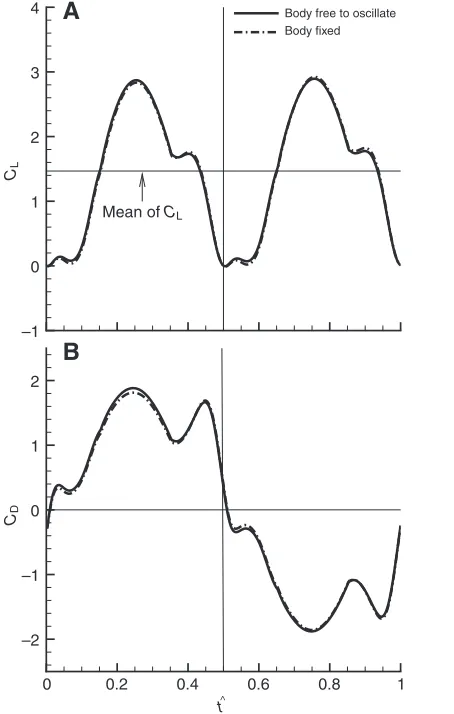
Fig. 9 gives the time courses of the lift (CL) and drag (CD)
coefficients of the wing in one cycle for the hovering dronefly, with and without body oscillations, the forces are non-dimensionalized by 0.5πU2S, where Sis the area of one wing. Fig. 10 gives the results for the hawkmoth.
Let us look at the results of the hawkmoth first (Fig. 10). For the wing lift (Fig. 10A), in some parts of the cycle (t⬇0 to 0.25;t⬇0.5 to 0.7), CLin the case with body oscillations is slightly larger than
that without body oscillations, and in other parts of the cycle (t⬇0.25 to 0.5;t⬇0.7 to 1.0), CLin the case with body oscillations is slightly
smaller than that without body oscillations. Thus the mean vertical force (mainly contributed by CL) is the same for the cases with and
without body oscillations, as it should be for balancing the weight. For the wing drag (Fig. 10B), in the whole cycle, the magnitude of
CDin the case with body oscillations is larger (by about 10%) than
that without body oscillations. This is because the angle of attack of the wing in the case with body oscillations is larger than that
–1 0 1 2
3
4 Body free to oscillate
Body fixed
A
Mean of CL
–2 –1 0 1 2
B
0 0.2 0.4 0.6 0.8 1
CL
CD
t^
Fig. 9. Time courses of lift and drag coefficients of a wing in one cycle for the dronefly with and without body oscillation. CLand CD, lift and drag
coefficients of the wing, respectively;t, non-dimensional time.
Table 4.αd, αuand needed for hovering (deg.)
DF HM
αd αu αd αu
Body fixed 31.8 31.8 2.8 38.3 39.5 11
Body free to oscillate 32.5 32.5 2.8 42.0 42.3 10.5
DF, model dronefly; HM, model hawkmoth; αdand αu, angles of attack of
[image:9.612.335.562.352.709.2]3322
without body oscillations. The larger wing drag would result in a larger power requirement (see below).
For the dronefly (Fig. 9), the force coefficients have rather small differences between the cases with and without body oscillations. This is expected from the above results that the body oscillations of the dronefly are very small.
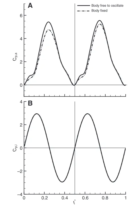
Effect on power requirements
Based on the aerodynamic forces and the kinematic and morphological data, the mechanical power required for the flight can be computed [for the computational method, see for example Fry et al., or Liu and Sun (Fry et al., 2005; Liu and Sun, 2008)]. Fig. 11 gives the instantaneous non-dimensional aerodynamic power,
Cp,a, and inertial power, Cp,i, of a wing in one cycle for the model
dronefly (the power is non-dimensionalized by 0.5ρU2Sc), for the cases with and without body oscillations. Fig. 12 gives the results for the model hawkmoth.
From Cp,aand Cp,i, the mass-specific power (the mean mechanical
power over a wingbeat cycle divided by the mass of the insect) can be calculated. In the case of zero elastic energy storage, the specific power is denoted as P1*, and in the case of 100% elastic energy
storage, as P2*. The calculated results are given in Table 5. For the
model hawkmoth, when the body is free to oscillate, the specific power is about 9% larger than that in the case without body oscillations. For the model dronefly, the corresponding value is about 2%.
Experimental and computational studies neglecting body oscillations
In previous experimental and computational studies on insect aerodynamics (e.g. Ellington et al., 1996; Dickinson et al., 1999; Sane and Dickinson, 2001; Sun and Tang, 2002a; Sun and Tang, 2002b; Berman and Wang, 2007), body oscillations were neglected. The above results show that for the hawkmoth, which has a relatively low wingbeat frequency and a large ratio of wing mass to body mass, when the body oscillations are included, the aerodynamic forces and power requirements differ by about 10% from that in the case of neglecting the body oscillations. But for the dronefly, which has a relatively high wingbeat frequency and small ratio of wing mass to body mass, the differences are rather small (about 2%).
As shown above, the motion of the body centre of mass in the horizontal direction dominates the body oscillation; and the non-dimensional horizontal displacement of the body centre of mass consisted of two parts, one (due to wing aerodynamic force) proportional to 1/cn2 and the other (due to wing inertial force) proportional to the ratio of wing mass to body mass. Ellington, Ennos, and Willmott and Ellington obtained morphological data and hovering kinematic data for many insects [more than 20 species from 6 orders (Ellington, 1984a; Ellington, 1984b; Ennos, 1989a; Willmott and Ellington, 1997a; Willmott and Ellington, 1997b)]. These data show that hawkmoths are among those insects which have the largest values of 1/cn2and wing mass to body mass ratio
(nis about 25 Hz and wing mass to body mass ratio is about 6%). For many insects, their nis several times larger and the wing mass to body mass ratio several times smaller than that of the hawkmoth. For those insects, the differences in aerodynamic forces and power
J. H. Wu, Y. L. Zhang and M. Sun
–1 0 1 2
3
4
A
–3
–2 –1 0 1 2
3
B
Body free to oscillate Body fixed
Mean of CL
0 0.2 0.4 0.6 0.8 1
CL
CD
t^
Fig. 10. Time courses of lift and drag coefficients of a wing in one cycle for the hawkmoth with and without body oscillation. CLand CD, lift and drag
coefficients of the wing, respectively; t, non-dimensional time.
0 2 4
A
–6 –4 –2 0 2 4
6
B
Body free to oscillate Body fixed
0 0.2 0.4 0.6 0.8 1
Cp,
a
Cp,i
t^
Fig. 11. Time courses of power coefficients in one cycle for dronefly, with and without body oscillation.Cp,a, aerodynamic power; Cp,i, inertial power;
3323 Hovering of model insects
requirements between the cases with and without body oscillations would be much less than 10%. As a result, it can be said that for many insects, when studying their hovering aerodynamic forces and power requirements, it is reasonable to neglect the body oscillations.
The present results are useful to flight stability and control analysis
Flight dynamic stability and control are of great importance in the study of the biomechanics of insect flight. Flight dynamic stability deals with the perturbed motion of a flying body about its equilibrium state following a disturbance; if the perturbed motion decreases with time and goes to zero, the flight is stable; otherwise, it is unstable or neutrally stable. Flight control has two aspects. One is stabilization control, which deals with applying active control to
stabilize the flight that is unstable or weakly stable; the other is control to change from one equilibrium state to another. Both the stability analysis and the control analysis need to start from the equilibrium state. The present method has provided the equilibrium state for hovering flight; it can also be used for obtaining periodic solutions of other flight modes (e.g. forward flight). In addition to finding the periodic solutions of equilibrium state, the integration process of coupling the equations of motion with the Navier–Stokes equations can be used to study the stability and control problems. But it should be noted that in the stability and control problems, lateral and forward translation and rotations about three axes of the body would occur, and the 6 degrees of body dynamics need to be considered, and, furthermore, the aerodynamic interactions of wing–wing and wing–body could become important. The dynamic equations in the present study (Eqn 1) are of 6 degrees of freedom. However, the Navier–Stokes solution might need to be modified to include the wing–wing and wing–body interaction effects.
Recently, some studies on flight dynamic stability and control were conducted using a simplified approach (e.g. Taylor and Thomas, 2003; Sun and Xiong, 2005). Two basic assumptions were made in the approach. The first was the ‘rigid body’ assumption; it assumed that the frequency of the perturbed motion of the body was much lower than the wingbeat frequency and effects of the flapping wings on the flight system could be represented by the wingbeat-cycle average aerodynamic and inertial forces. The second assumption was that linearization of the equations of motion was applicable. The validity of those assumptions needs to be tested, and this can be done by methods which solve the equations of the full non-linear systems.
Some discussion on the solution method and the effects of variations in wing kinematics
The validity of the solution method
A major assumption of the solution method is that the historical wake of the flapping wing before the period of solution (t=0 to t=T) can be approximated by that in the case without body oscillations. Now that we have obtained the periodic solutions of the body motion, we can examine the validity of the assumption as follows. We make two flow computations. In the first one (case A), from
t=–3T to t=T, the model hawkmoth oscillates according to the periodic solution functions, ub(t), wb(t), qb(t) and θb(t), obtained
above. In the second computation (case B), fromt=–3Ttot=–0.1T, the body is fixed [ub(t)=wb(t)=qb(t)=0, θb(t)=χ]; from t=–0.1T to t=0, ub(t), wb(t), qb(t) and θb(t) change smoothly to ub(0), wb(0), qb(0) and θb(0) of case A, respectively; from t=0 to t=T, ub(t), wb(t), qb(t) and θb(t) are the same as those of case A (Fig. 13). The flapping
motion of the wing, started at t=–3T, is the same for the two cases. The validity of the assumption can be examined by comparing the computed aerodynamic forces in the cycle from t=0 to t=Tof the two cases. Fig. 13E shows the comparison. The results of the two cases are almost identical (in Fig. 13, only the comparison of CLis
given; comparisons of CDand CMbetween the two cases are similar),
showing that the assumption is reasonable.
A further test is done by another two computations (called case a and case b). In case a, the body motion is similar to that of the above case A, except that the amplitudes of the oscillations are doubled. In case b, fromt=–3Ttot=–0.1T, the body is fixed; from
t=–0.1Ttot=0, ub(t), wb(t), qb(t) and θb(t) change smoothly to ub(0), wb(0), qb(0) andθb(0) of case a, respectively; and from t=0 to t=T, ub(t), wb(t), qb(t) and θb(t) are the same as those of case a. The
computed aerodynamic forces in the cycle from t=0 to t=Tare given in Fig. 14. Only a very small difference is seen between the two
0 2 4 6
A
–4 –2 0 2
4
B
Body free to oscillate Body fixed
0 0.2 0.4 0.6 0.8 1
Cp,
a
Cp,i
t^
Fig. 12. Time courses of power coefficients in one cycle for hawkmoth, with and without body oscillation.Cp,a, aerodynamic power; Cp,i, inertial power;
t, non-dimensional time.
Table 5. Specific power for hovering (W kg–1)
DF HM
P1* P2* P1* P2*
Body fixed 63.91 38.55 40.83 35.61
Body free to oscillate 64.72 39.46 44.34 39.01
DF, model dronefly; HM, model hawkmoth; P1* and P2*, specific power with
[image:11.612.49.272.66.425.2]3324
cases. This shows that even if the body oscillations are twice as large as those of the model hawkmoth, the assumption is still reasonable.
As discussed above, the hawkmoth has a relatively low wingbeat frequency and a large ratio of wing mass to body mass. If the assumption is valid for body oscillations twice as large as that of the hawkmoth, it is expected that it is valid for many insects; it should be noted that for insects with rather large body oscillations, e.g. many butterflies [their velocity of body oscillation is comparable to wing flapping velocity (see Dudley, 1990)], the assumption would not be valid.
Effects of variations in wing kinematics
Idealized representations of wing kinematics are used in the present study, e.g. the out-of-plane motion of wing (deviation) is not included and the positional angle of the wing is approximated by the simple harmonic function. Here we make an additional computation for the hawkmoth to examine the effects of the approximations of wing kinematics on the solutions, by using the realistic wing kinematics (suggested by a reviewer of this paper).
Let the above computation for the hawkmoth [moth M1 in Willmott and Ellington (Willmott and Ellington, 1997a; Willmott and Ellington, 1997b)] be known as case 1. There the positional angle φ(t) is the simple harmonic function, the deviation angle θ(t) is zero and the wing rotation time during the stroke reversal is 0.3T. The results of case 1 have been given above (Fig. 8).
The additional computation is known as case 2, in which more realistic wing kinematics is to be used. For the hawkmoth [moth M1 in Willmott and Ellington (Willmott and Ellington, 1997b)], only the time course of α(t) is available in Willmott and Ellington’s paper. The time courses of φ(t) and θ(t) for this moth are available in another paper of Ellington and colleagues (Liu et al., 1998); they are replotted in Fig. 15A (the curves were based on the first three Fourier series terms, which were fitted to the measurements by Willmott and Ellington). φ(t) and θ(t) in Fig. 15A are used in case 2. As for α(t), we still assume it is constant in the mid-downstroke (denoted as αd) and in the
mid-upstroke (denoted as αu), and during stroke reversal it is modeled
by Eqn 10. The rotation time, determined from Willmott and
J. H. Wu, Y. L. Zhang and M. Sun
A
Case ACase B
B
C
–3 –2 –1 0 1
D
–1 0 1 2
3
4
E
0 0.2 0.4 0.6 0.8 1
CL
–0.06 0 0.06
θb –0.06
0 0.06
qb
*
–0.06 0 0.06
z
. E,b
/
U
–0.06 0 0.06
x
. E,
b
/
U
t/T
Fig. 13. Time courses of body motion variables of case A and case B in the four cycles (fromt=–3T to t=T), and comparison of lift coefficient (CL) in the
fourth cycle (fromt=0 to t=T) between case A and case B. xE,b/U and zE,b/U, non-dimensional horizontal and vertical velocities of body centre of
mass, qb*, non-dimensional pitch rate of body; θb, pitch angle; t, time; T,
wingbeat period.
–1 0 1 2
3
4
Case a
Case b
0 0.2 0.4 0.6 0.8 1
CL
t/T
Fig. 14. Comparison of lift coefficient (CL) in the fourth cycle (from t=0 to
3325 Hovering of model insects
Ellington’s data [see figure 10B in Willmott and Ellington (Willmott and Ellington, 1997a)], is 0.3Tfor the supination and 0.2Tfor the pronation. The values of αd, αuand are adjusted
to ensure the force and moment balance. The time derivatives of φ, θand αare shown in Fig. 15B.
The computed results of case 2, compared with those of case 1, are given in Fig. 16. It can be seen that the main motion, i.e. the relatively large horizontal oscillation (xE,b), is changed only a little by the wing kinematics change (Fig. 16A), whilst the relatively small motions, the vertical oscillation (zE,b) and the body pitch oscillation (qb,Δθb) are changed considerably by the wing kinematics change
(Fig. 16B,C,D).
Fig. 17Ai, Bi and Ci shows the time course of the horizontal and vertical forces and pitching moment acting on the insect (coefficients CH, CV and CM denote the non-dimensional
horizontal and vertical forces and pitching moment, respectively). The forces and moment are contributed by the aerodynamic and inertial forces and moment of the flapping wings. Fig. 17Aii and Aiii, Bii and Biii and Cii and Ciii shows the contributions from the aerodynamic and inertial forces and moments of the flapping wings. It is seen that variation in wing kinematics affects the aerodynamic forces and moments, as well as the inertial forces and moments of the wings. From Fig. 17Ai, Bi and Ci, it can be seen that the horizontal force (CH) is much less affected by the
wing kinematics change than the vertical force (CV) and pitching
moment (CM). This is because the amplitude of oscillation of CH
is much larger than those of CVand CM, hence CHis less sensitive
to the wing kinematics change than CV and CM. This explains
why the main motion, i.e. the horizontal oscillation of the body, is much less affected by the wing kinematics change than the relatively small vertical oscillation and body pitch oscillation.
φ
,
θ
–60 –40 –20 0 20 40 60
80
A
φ θ
–1 –0.5 0 0.5 1
–3
–2 –1 0 1 2
3
B
φ*
,
θ*
.. α
*
.
α*θ*. . φ*.
0 0.2 0.4 0.6 0.8 1
t^
Fig. 15. (A) The time courses of the positional angle (φ) and deviation angle (θ) in one cycle [plotted using data from Liu et al. (Liu et al., 1998)]. (B) The time courses of the non-dimensional time derivative of the positional angle (*), derivation angle (*) and angle of attack (␣*); t, non-dimensional time.
–0.06 0
0.06
A
Case 2 Case 1
–0.02 0
0.02
B
–0.06 0
0.06
C
–0.04 0
0.04
D
z
. E,
b
/
Ux
. E,
b
/
U
φ=10.5 deg. αu=42.3 deg. αd=42 deg.
0 0.2 0.4 0.6 0.8 1
φ=11.9 deg. αu=36.2 deg. αd=40.1 deg.
qb
*
Δθb
t^
Fig. 16. Effects of varying wing kinematics. xE,b/U and zE,b/U,
non-dimensional horizontal and vertical velocities of the body centre of mass; qb*, non-dimensional pitch rate; Δθb, pitch angle minus its mean value; αd
and αu, angles of attack of the wing in the downstroke and upstroke,
3326
APPENDIX A
For any vector V, in frame (xE,yE,zE) (see Fig. 1), we write:
where VxE, VyE and VzEare the xE,yE and zEcomponents of V,
respectively. Similarly, in frame (xb,yb,zb) and frame (xw,yw,zw):
where Vxb, Vyb and Vzb are the xb, yb and zb components of V,
respectively, and Vxw, Vywand Vzware the xw, ywand zwcomponents
of V, respectively. EV, bVand wVare related by the following (Sun
et al., 2007):
Here bErE, wErE and wErb are matrix of direction cosines. For example, bErEis determined by ψb, θband φb, the Euler angles
relating frame (xb,yb,zb) to frame (xE,yE,zE);wErbis determined by
ψw, θwand φw, the Euler angles relating frame (xw,yw,zw) to frame
(xb,yb,zb) (see Sun et al., 2007). With respect to the inertial frame,
EV= E b→EbV
,EV= E w→EwV
and bV= E w→bwV
. (A3)
ν ν ν ν ν ν ν
EV= VxE VyE VzE ⎡ ⎣ ⎢ ⎢ ⎢ ⎤ ⎦ ⎥ ⎥
⎥ , (A1)
ν
ν ν
ν
ν
ν ν
bV= V xb V yb V zb
⎡ ⎣ ⎢ ⎢ ⎢ ⎤ ⎦ ⎥ ⎥
⎥ and wV=
V xw V yw V zw
⎡ ⎣ ⎢ ⎢ ⎢ ⎤ ⎦ ⎥ ⎥ ⎥ , (A2) ν ν ν ν ν ν ν
the centre of mass of the wingless body moves at velocity vcg,
the body rotates at angular velocity ωbd and a wing rotates at
angular velocity ωwg(since angular velocity of the wing relative
to the body is prescribed, ωwgis related toωbdas ωwg=ωbd+ωwg,0,
where ωwg,0is the angular velocity of the wing relative to the
body). Rcgis the position vector of the centre of mass of the body; Rhis the vector from the body centre of mass to the root of a
wing; Rwgis the vector from the root of a wing to the centre of
mass of the wing (Fig. 1). LetFAbe the total aerodynamic force
and MAthe total aerodynamic moment about the centre of mass
of the body, mbthe mass of the insect body,mwgthe mass of a
wing, Ibd the matrix of moments and products of inertia of the
body, Iwgthe matrix of moments and products of inertia of a wing, gthe gravitational acceleration and tthe time. The equations of motion [equations 6 and 7 in Sun et al. (Sun et al., 2007)] are as follows:
ν
ν ν
ν
ν bFA+ mb+ mwg,i
i=1
N
∑
⎡ ⎣ ⎢ ⎢ ⎤ ⎦ ⎥⎥bg= mb+i=1mwg,i
N
∑
⎡ ⎣ ⎢ ⎢ ⎤ ⎦ ⎥ ⎥dbνcg
dt +bbd×bνcg
⎛ ⎝⎜
⎞ ⎠⎟
+ mwg
dbbd
dt ×bRh+bbd×
(
bbd× bRh)
⎡ ⎣ ⎢ ⎤ ⎦ ⎥ ⎧ ⎨ ⎪ ⎩⎪ ⎫ ⎬ ⎪ ⎭⎪i i=1
N
∑
+ mwg E w→b
dwwg
dt ×wRwg+wwg×
(
wwg×wRwg)
⎡ ⎣ ⎢ ⎤ ⎦ ⎥ ⎧ ⎨ ⎪ ⎩⎪ ⎫ ⎬ ⎪ ⎭⎪i i=1
N
∑
, (A4)J. H. Wu, Y. L. Zhang and M. Sun
0 2 4 6 8
Ai
–4 –2 0 2 4Aii
–6 –4 –2 0 2 4 6Aiii
–4 –2 0 2 4 6 –4 –2 0 2 4 –4 –2 0 2 4 –2 0 2 –4 –2 0 2 4 –4 –2 0 2 40 0.2 0.4 0.6 0.8 1 0 0.2 0.4 0.6 0.8 1
0 0.2 0.4 0.6 0.8 1
Mean of CV
CH,i CH,
a
CH
Case 2 Case 1
–6 –8 –4 –2
Biii
Bii
0 0.2 0.4 0.6 0.8 1
Bi
Mean of CV,a
CV,i CV,
a
CV
0 0.2 0.4 0.6 0.8 1
Ciii
Cii
Ci
CM,i CM, a CM0 0.2 0.4 0.6 0.8 1
0 0.2 0.4 0.6 0.8 1
t^ t^ t^
Fig. 17. Time courses of the coefficients of the horizontal and vertical forces and pitching moment in one cycle. CHand CV, horizontal and vertical force
coefficients, respectively;CM, pitching moment coefficient; CH,a, CV,aand CM,a, contributions by the aerodynamic force of the wing; CH,i, CV,iand CM,I,
contributions by the inertial force of the wing; t,non-dimensional time.
3327 Hovering of model insects
where Nis the number of wings (in the present study, N=2). The unknown variables in the equations of motion (Eqns A4 and A5) are νcgand ωbd(n