DOI:10.1051/0004-6361/201116652 c
ESO 2013
Astrophysics
&
Coronal heating and nanoflares: current sheet formation
and heating
R. Bowness, A. W. Hood, and C. E. Parnell
School of Mathematics and Statistics, University of St Andrews, North Haugh, St Andrews, Fife, KY16 9SS, UK e-mail:[email protected]
Received 4 February 2011/Accepted 14 November 2013
ABSTRACT
Aims.Solar photospheric footpoint motions can produce strong, localised currents in the corona. A detailed understanding of the formation process and the resulting heating is important in modelling nanoflares, as a mechanism for heating the solar corona. Methods.A 3D MHD simulation is described in which an initially straight magnetic field is sheared in two directions. Grid resolutions up to 5123 were used and two boundary drivers were considered; one where the boundaries are continuously driven and one where
the driving is switched offonce a current layer is formed.
Results.For both drivers a twisted current layer is formed. After a long time we see that, when the boundary driving has been switched off, the system relaxes towards a lower energy equilibrium. For the driver which continuously shears the magnetic field we see a repeating cycle of strong current structures forming, fragmenting and decreasing in magnitude and then building up again. Realistic coronal temperatures are obtained.
Key words.magnetohydrodynamics (MHD) – magnetic reconnection – Sun: corona
1. Introduction
The Sun’s corona is much hotter than its visible surface: the pho-tosphere’s average temperature is 6000 K compared to over a million K in the corona. Back in 1974,Levine(1974) proposed a new theory for heating the corona involving the dissipation of many tiny little current sheets, which built on the resistive insta-bility ideas first proposed byParker(1972). This heating theory is better known today as nanoflare heating and was developed in a series of papers by Parker (Parker 1987,1988). Various ob-servational papers (e.g.,Krucker & Benz 2000;Parnell & Jupp 2000;Vekstein & Jain 2003) and theoretical papers (e.g.,Cargill 1993; Cargill & Klimchuk 1997, 2004; Klimchuk & Cargill 2001) lend support to this idea, but there are still many open questions. In particular, in Parker’s nanoflare heating theory the strong, localised currents in the solar corona were produced by the braiding of magnetic fields whose photospheric footpoints are moved about by convective motions. Although there are a multitude of magnetic features with a wide range of fluxes (Schrijver & Zwaan 2000;Parnell et al. 2009) which are con-tinuously emerging, moving, cancelling, fragmenting and coa-lescing (Schrijver et al. 1997), it is unclear whether the braiding motions envisaged by Parker really do occur.
Tangential discontinuities, or current sheets (current layers) as they are better known, are regions where the gradient of the magnetic field and, therefore, the electric currents are very large. These currents may then dissipate due to a resistive instability, leading to magnetic reconnection, which allows the field lines to break and reconnect with some of the magnetic energy being released as heat. An aim of this paper is to follow the formation and break-up of current layers and investigate the flow of energy from the footpoint motions into the magnetic field and, through the conversion of magnetic energy, into heat in the regions of strong current. This paper investigates the heating of the plasma at the site of a single heating event.
It is well known that current layers can form at null points in both two dimensions (e.g. Green 1965; Syrovatskiˇı 1971; Bungey & Priest 1995; Craig & Litvinenko 2005; Fuentes-Fernández et al. 2011) and three dimensions (e.g., Rickard & Titov 1996; Pontin & Craig 2005; Pontin et al. 2007a,b;Masson et al. 2009;Priest & Pontin 2009;Al-Hachami & Pontin 2010;Fuentes-Fernández & Parnell 2012,2013). They also develop at other topological features such as separators (e.g.,Lau & Finn 1990;Longcope & Cowley 1996;Priest et al. 2005;Haynes et al. 2007;Parnell et al. 2010a) and separatrix surfaces (e.g.,Priest et al. 2005;Mellor et al. 2005;De Moortel & Galsgaard 2006a,b). However, they may also develop at ge-ometrical features, such as quasi-separatrix layers (e.g.,Priest & Démoulin 1995;Démoulin et al. 1996;Aulanier et al. 2006; De Moortel & Galsgaard 2006a,b;Wilmot-Smith & De Moortel 2007). Indeed, a considerable body of work also exists on the formation and dissipation of current layers in initially simple fields that have been driven in a variety of different ways through shearing or rotating motions or through compressive motions (e.g.,Galsgaard & Nordlund 1996a;Browning et al. 2008;Hood et al. 2009;Janse & Low 2009;Bhattacharyya et al. 2010;Huang et al. 2010).
Recently, using reduced magnetohydrodynamics (MHD), Rappazzo et al.(2007,2008,2010) have investigated the forma-tion and evoluforma-tion of current sheets and the cascade of energy to small-scales. In their system which is continuously driven at the photospheric boundary, they study the turbulent cascade of en-ergy injected at large photospheric scales down to its dissipation at numerous current layers at the small scale. In their simula-tions, the energy equation is replaced by∇⊥·u⊥ =0. This means there is no information about the thermodynamic response due to any loss of magnetic energy. Here, we investigate the formation and dissipation of a single current structure using full 3D MHD, where energy is conserved if the resistivityηis greater than the numerical dissipation.
Gudiksen & Nordlund(2006) produced a model of the com-plete solar atmosphere. They imposed an observed velocity pat-tern on the photosphere and showed that all the Poynting flux injected into the corona is dissipated. However, the scale of the simulation meant that individual energy release sites were not fully resolved and so it was not possible to identify the loca-tions and nature of these energy release sites. Recently though, a detailed analysis of the currents and reconnection in a numer-ical model of flux emergence has revealed that a complex web of separators through the current accumulations are responsible for the reconnection of newly emerged flux into the solar atmo-sphere with an overlying coronal magnetic field (Parnell et al. 2010b).
In this paper, we investigate the evolution of an initially straight magnetic field, which has first been sheared analyti-cally and relaxed to an equilibrium. This field is then stressed by shearing motions on two boundaries similar to the models of Longbottom et al.(1998) and Galsgaard & Nordlund(1996b). Unlike inLongbottom et al.(1998), where a magnetic relaxation technique is used, our experiments use a 3D MHD code. Due to the considerable advancements in computing hardware over the past 15 years, we run simulations with grid resolutions of 5123. These are of a much higher resolution than the maximum of 1363 achieved inGalsgaard & Nordlund(1996b). Another difference toGalsgaard & Nordlund(1996b) is that we do not consider multiple random shearing of the uniform field, instead just two shears are preformed in our experiments. These create a single initial current layer, as opposed to the many transient current ac-cumulations seen inGalsgaard & Nordlund(1996b),Rappazzo et al.(2010) andDahlburg et al.(2012). By looking closely at the energetics of our single current layer system we investigate whether the dissipation of such a layer provides sufficient energy for either a single nanoflare on its own or many nanoflares when the system is continuously driven. Hence, we aim to determine if these types of current layers really can be the building blocks of coronal heating and, if so, what the characteristics and properties are of these building blocks.
The numerical code, basic equations and boundary condi-tions used in this paper are described in Sect. 2. The model is based on two shears; the first shear is described in Sect. 3 and the second shear is discussed in Sect. 4. Subsequently the evolu-tion of the magnetic field (Sect. 5), the energetics (Sect. 6) and the current layer structure (Sect. 7) are analysed. A discussion of the results and general conclusions can be found in Sect. 8.
2. Numerical model
The simulations are carried out using the 3D MHD, Lagrangian remap, shock capturing code Lare3d (described in detail in Arber et al. 2001). The Lagrangian step is a straight forward predictor-corrector scheme and is fully 3D. After the Lagrangian step, the variables are remapped, preserving conserved quanti-ties, onto the original grid. Artificial viscosity is used to deal with shocks and van Leer gradient limiters (van Leer 1979) are applied at the remap step to preserve monotonicity, with the ap-propriate shock heating applied to the energy equation. The nu-merical grid is staggered so that: the density, pressure and spe-cific internal energy density are defined at the cell centres; the velocities at the vertices; the magnetic field components at the cell faces and the current components along the edges of the nu-merical cell. The staggered grid reduces the amount of averaging required in some of the calculations, thus reducing the associated error, and avoids the chequerboard instability. Further details of the code can be found inArber et al.(2001).
2.1. MHD equations
The resistive MHD equations are ∂ρ
∂t =−∇.(ρu), (1)
Du Dt =
1 ρj×B−
1
ρ∇P, (2)
∂B
∂t =−∇ ×E, (3)
ργ (γ−1)
D Dt P ργ
=ηj2, (4)
E+u×B=ηj, (5)
∇ ×B=μ0j, (6)
whereBis the magnetic field, jis the current density,uis the velocity, Eis the electric field, Pis the plasma pressure,γ = 5/3 is the ratio of specific heats,ρis the mass density,ηis the resistivity andμ0is the magnetic permeability andtis time.
Lare3druns with a normalised versions of these equations, where the normalisation is through the choice of normalising magnetic fieldB0, densityρ0and lengthL0. Thus, we define di-mensionless quantities asx=L0xˆ,B=B0Bˆ andρ=ρ0ρˆ. These three basic normalising constants are then used to define the nor-malisation for velocity, pressure, time, current density, electric field and temperature through
v0 = B0 √μ
0ρ0,
P0= B2
0 μ0,
t0= L0 v0,
j0 = B0 μ0L0
, E0=v0B0, T0 = ˜ μv2
0
R , (7)
so thatu = v0uˆ, j = j0ˆj,t = t0tˆandP = P0Pˆ. The magnetic permeability isμ0=4π×10−7H m−1, ˜μ=0.5 and the gas con-stant isR=8.3×10³m2s−2K−1. The resistivity is normalised through
ˆ
η= η
μ0L0v0
, (8)
orη0 = μ0L0v0. Since v0 is the normalised Alfvén speed this means that ˆη=1/S, whereS is the Lundquist number.
Dropping all of the hats on the normalised variables the final normalised resistive MHD equations, in Lagrangian form, are
Dρ
Dt =−ρ∇.u, (9)
Du Dt =
1
ρ(∇ ×B)×B− 1
ρ∇P, (10)
DB
Dt =(B.∇)u−B(∇.u)− ∇ ×(η∇ ×B), (11) D
Dt =− P ρ∇.u+
η
ρj2, (12)
where=P/ρ(γ−1) is the specific internal energy density. Note that, if∇.B=0 is initially satisfied, it remains at round-offerror throughout.
We neglect gravity in our simulations and initially setρ=1 and = 0.01, corresponding to a gas pressure of 0.00667 and plasma β of 0.013. The physical viscosity is set to zero, but Lare3dalso uses an artificial viscosity to deal with shocks and includes the corresponding shock heating in (12).
In a solar context, if we choose the unit of magnetic field strength B0 = 10 G, the electron number density ne = 5× 10¹⁴m−3 and the unit of lengthL
a short loop over the top of a single supergranule cell), we have normalising values of velocityv0=975.5 km s−1, timet0 =51 s and temperatureT0=5.7×10⁷K.
2.2. Resistivity
The resistivity,η, is varied depending on the aim of the exper-iment. In the solar corona, the typical values ofη are in gen-eral believed to be less than 10−10m2s−1. Since such values are not achievable in today’s numerical experiments, we choose the smallest possible value ofηwe can. This is done by settingη=0 and thus assuming an ideal evolution of the field. However, as will be shown in Sect. 6, even in this case we still get some re-connection. This is because when very fine scales are formed numerical diffusion occurs which results in reconnection. The consequences for the evolution and energetics of this numerical dissipation of the current sheet are discussed in detail in Sect. 6. We also perform a series of resistive MHD experiments in which constant normalisedηvalues of 10−5 and 10−4 are used. These experiments are compared with those of the “ideal” MHD runs in order to determine the effects of resistivity on the for-mation of the current layer and to follow the energetics of the system. The choice ofηhas implications for conservation of en-ergy; too small and numerical dissipation can be important.
2.3. Boundary conditions
The equations are solved in a 3D Cartesian box,−w < x < w, −w < y < wand−L<z<L. As inLongbottom et al.(1998), we setw=0.3,L =0.5. We assume periodic boundary conditions in bothxandy(the sides of the box) and the boundary atz=±L is line-tied (the top and base of the box). The magnetic field components, specific internal energy density and mass density on the top and bottom boundaries have zero normal derivative, i.e. ∂Bx
∂z = ∂By
∂z = ∂Bz
∂z = ∂∂z = ∂ρ
∂z = 0. On the top and bottom boundaries, the components of the velocitiesvyandvzare both set to zero andvxis discussed later in Sect. 4.
3. Initial magnetic field: first shear
The initial magnetic field we will use in our numerical simu-lations already includes a first shear and is analytically derived below. However, we also discuss a numerical experiment imple-menting the first shear in order to confirm our approach of start-ing from the analytical magnetic field derived and to demonstrate the limitations that should be imposed on the speed of the driver to ensure the intended displacement.
We assume the initial magnetic field has been reached by ideal MHD after a first sinusoidal shear. Such a state can be derived analytically as shown below. This initial state was also reached numerically byLongbottom et al.(1998). Assuming that the field has been sheared and that is has relaxed to an equilib-rium, we can model this by considering a flux function
A=[0,A(x,z),0]. (13)
The first shear will be in theydirection, as inLongbottom et al. (1998). So although there is no variation in theydirection, this shear will introduce aycomponent to the magnetic field, so we have
B=
−∂A∂z,By(A),∂A ∂x
· (14)
The resulting force-free field satisfies the 2D Grad-Shafranov equation
∇2A+B
y(A)ddBAy =0. (15) Previous work, most notably that byLothian & Hood(1989) and Browning & Hood(1989), helps to simplify our model.Lothian & Hood(1989) looked at the effect of a small twist on magnetic flux tubes. For a cylindrical loop that is much longer than it is wide, they showed that variations in the axial direction can be neglected, apart from boundary layers near the two footpoints. Hence, a theory was developed, based on straight loops with a constant cross sectional area, to show that the main properties of the loop could be explained by a simple 1D model rather than solving the 2D Grad-Shafranov equation.Mellor et al. (2005) used this idea to analytically verify the location of current accu-mulations when two sources are moved relative to two stationary sources. Using the approach ofMellor et al.(2005), we see that the flux function can be approximated by a function ofxalone.
Therefore, we assume an initial magnetic field of the form B=[0,By(x),Bz(x)], (16) where, in order to satisfyj×B=0, we have
B2y+B2z =constant. (17)
As inGalsgaard & Nordlund (1996b), we choose a sinusoidal shear profile forBy(x), withBz(x) chosen to satisfy Eq. (17). B=
⎡
⎢⎢⎢⎢⎣0, λsin πx w
, 1+λ2cos2 πx
w⎤⎥⎥⎥⎥⎦· (18)
We can now calculate the footpoint displacement that generates these magnetic field components. The exact profile of the first shear is not important. All that is necessary is that the first shear produces sheared fields. Thus, the first shear we actually impose is given by
L
−L dz Bz(x) =
d
−d dy By(x)
which, after integrating, gives the footpoint displacement as d= LBy(x)
Bz(x) ·
(19) For our simulations, withL =0.5 andBy,Bz, as defined above, the displacement is
d= Lλsin πx
w
1+λ2cos2πx w
Lλsin πx w
forλ <1. (20)
As we shear on both the top and bottom boundaries, but in op-posite directions, the overall maximum footpoint displacement isD=2max(d)=2λL.
Hence, as we have L = 0.5 andw = 0.3, we find that the maximum shear displacement is equal to the value of λ. The particularλused is given in the next section when implementing the second shear.
Although we present results here with the first shear taken analytically, we have also investigated it numerically by start-ing from a vertical magnetic field (shear parameterλ =0) and implementing a driving profile of
vy(x, y,∓L)=±V0 2 sin
πx w tanh
t−t1
td
−tanh
t−t2 td
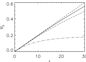
Fig. 1.Maximum value ofByas a function of time with 1283grid points.
Dashed curve is the ideal MHD case. Solid curve isη = 10−5,
dot-dashed curve isη=10−4and triple dot-dashed curve isη=10−3.
wheret1is the time the driver ramps up,t2is the time the driver starts to reduce back to zero andtd is the duration over which the driver is ramped up or down. So the driving ramps up to a maximum normalised speed ofV0before reducing back to zero. This means that the footpoint displacement reaches a maximum value and does not increase after that.
Importantly we note that the first shear does not excite any instabilities and there is no evidence of tearing. The Lare code has been used for reconnection studies and has successfully in-vestigated tearing modes with both uniform and non-uniform re-sistivity.
The dominant velocity component is given by vy = V0zsin(πx/w))/Land this generatesBy = By(t) sin(πx/w). The ycomponent of the induction equation can be expressed as ∂By
∂t = V0
L Bz− ηπ2
w2 By. (22)
We can illustrate the evolution of the maximum ofByas a func-tion of time by takingBz =B0 as a constant. Ifη =0, then we simply have the maximum ofBygiven by
By(t)=B0 V0t
L =B0 d
L, (23)
whered =V0tis the distance the footpoints have been sheared and from Eq. (20) our parameterλ = d/L. However, ifη 0, then the solution (as also shown byRappazzo et al.(2010)) is By= B0V0w
2
Lηπ2
1−e−ηπ2t/w2= B0 Lη˜
1−e−η˜d, (24) where ˜η=ηπ2/V
0w2. Figure1showsBy(t) for three values ofη and for ideal MHD. Obviously, if ˜ηdis small, then solution (24) agrees with the ideal evolution of (23). However, this assump-tion that ˜ηdis small depends on the choices for bothηandV0. The comparison between the numerical solution from the Lare code for the maximum ofByas a function of time and the ap-proximation given by Eq. (24) is exceptionally good.
During the first shear, there are no small length scales gen-erated and the choice of the value ofηis not restricted by the need to resolve any strong current regions. Choosingη =10−5, we have conservation of total energy. WithL = 0.5, w = 0.3 andV0 = 0.01, we have ˜η = 0.1 and, for t = 25, we have d = 0.25. Hence, the maximum of By will be approximately given by 0.45, rather than by 0.5 had the evolution been under ideal MHD. However, forη=10−3, the maximum ofB
y=0.17. Thus, there is significant resistive slippage of the field lines for this choice ofη and the field is not as sheared as expected. In
fact, regardless of how long the shearing motions are applied the maximumBycan reach is 0.18 forη=10−3.
One way to reduce this slippage, for a given footpoint dis-placement, is to increase the value ofV0. For example, increas-ingV0 by a factor of 5 means that, forη =10−3,By =0.36 for d=0.25.
The choice forηis not too important for the first shear, and a small value ofηis possible, but, it is important for the second shear as the transverse length scale,w, rapidly shortens when the current layer starts to form. The value ofηneeded must be increased (or the number of grid points increased significantly) to ensure that the layer is resolved and that energy is conserved. We show in Sect. 6.2 thatη=10−5is not large enough to resolve the dissipation within the current layer during the second shear but thatη=10−4is large enough for a 5123grid.
Now the speed of the shearing motion becomes important onceηis chosen for current sheet resolution. Too small a value forV0 and the evolution is not that intended from the driving velocity. Driving does not necessarily continue to increase the magnetic field components. Thus, we need to selectV0such that, as we stated above, the various timescales are well separated. Obviously on the Sun, the various timescales are well separated and the observed driving velocity is slow enough for sequences of equilibria but fast enough to exceed any resistive slippage. However, since computational experiments have the value ofη limited by grid resolution, the speed at which the boundaries are driven is chosen as a balance between computational time and a more realistic driving velocity.
The results from the numerical simulation for the first shear can be compared with our predicted form for By (Eq. (18)). Using η = 10−5, we obtain an excellent agreement with the equilibrium predictions of analytical studies such asBrowning & Hood(1989) and numerical studies such asMellor et al.(2005) andRappazzo et al.(2010).
4. Drivers: second shear
Next we drive a second shear in thexdirection by imposingvxon the top and bottom boundaries (positive direction on the bottom boundary and negative direction on the top boundary).
We choose the same type of sinusoidal shear profile as in Sect. 3,
vx(x, y,∓L)=±sin πy w
f(t), (25)
where f(t) is a function, discussed in detail below, determining how fast and how much the field is sheared. The actual displace-ment achieved with our second shear is found from integrating vxin time and then multiplying by two, as the shear is in oppo-site direction on the top and bottom boundaries. Hence, we have
D=2 sin πy w
t
0
f(τ)dτ. (26)
magnitude 0.8 was used and a possible current sheet was formed after a shear in the second direction of 0.6−0.7.
We run two sets of experiments which have the same spa-tial profiles in vx, but they have different temporal dependen-cies. The first set use driver 1, which continuously drives the boundaries throughout the simulation, while the second set use driver 2, which drives the boundaries up until a localised current layer forms and then the driver is switched off.
4.1. Driver 1
Driver 1 has a velocity profile that ramps up to a constant nor-malised value of 0.05, corresponding to a photospheric velocity of roughly 50 km s−1, namely
vx(x, y,∓L)=±0.025 sin πy
w 1+tanh
t−t1 td
, (27)
where t1 and td are chosen to be 2.0 and 0.5, respectively. This velocity is high compared with observed photospheric val-ues, but is necessary due to computational time constraints. Nonetheless, the velocity is still highly sub-Alfvénic and the magnetic field evolves slowly through a sequence of equilibria. Since the transit time for any waves propagating through the box is about one, in our dimensionless variables, they have time to settle down. Thus the evolution of the magnetic field, although sped up, will be equivalent to that found for much slower, more realistic, speeds.Mellor et al. (2005) andGalsgaard & Parnell (2005) have shown that, provided the driving speeds are slower than the Alfvén speed, it is the actual footpoint displacement that is important for the formation of current layers. The hyperbolic tanh profile is chosen so that we have a gradual rise up to our constant value. This prevents any impulsive motion at t = 0. Simulations with a slower shear were also performed. The max-imum ofBywas found to match for both shears up to a displace-ment of 0.2. The maximum of jz agreed up to a displacement of 0.15 and, beyond that, the faster shear had a smaller maxi-mum value. The maximaxi-mum value of the maximaxi-mum of jz, while different for the two shears, occurred at the same displacement of 0.22. So qualitatively, there was no significant different be-tween the two cases.
As already mentioned, driver 1 continuously drives the field at a constant value. Inevitably, whether we are using ideal or resistive MHD, reconnection will occur (due to either numerical diffusion or components of the induction equation). Since one of our aims is to look at the formation of a current layer we want to switch offthe driver at some time so we stop driving the field and stop injecting more energy. This enables us to investigate the current layer. Hence, we run a series of experiments using a second driver, driver 2.
4.2. Driver 2
The imposed boundary shearing motion in driver 2 has the same spatial profile as driver 1, but now has a temporal variation so that it rises to a maximum speed and then reduces back to zero, similar to the driving profile implemented in Sect. 3.
vx(x, y,∓L)=±0.025 sin πy w tanh
t−t1
td
−tanh
t−t2 td
,
[image:5.595.307.559.75.320.2](28) wheret1 andtd are chosen to be 2 and 0.5, respectively, as for driver 1. The value fort2is chosen to be 7 after a consideration
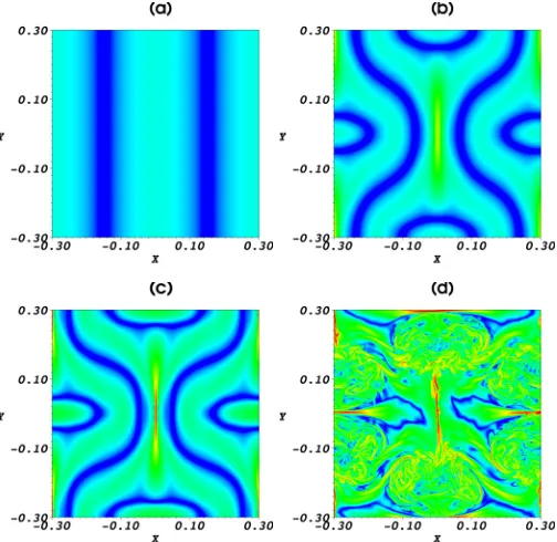
Fig. 2.Contour plots of the logarithm of the current magnitude in the mid-plane,z =0, for normalised times 0, 5, 7 and 10 (a)–d), respec-tively) for the experiment using driver 1,η=0 and with a grid resolu-tion of 5123. Red corresponds to a maximum of 400 while blue
corre-sponds to a minimum value of 1.
of the behaviour of the maximum current as shown below. Note that if t2 is too small, no current layer forms and there is no dynamic evolution.
5. Evolution of the magnetic field
As already explained, the uniform field is first sheared analyt-ically in thexdirection. A cut of the magnitude of the current in the mid-plane,z=0, shows that at this stage there is no real accumulation of current within the domain Fig.2a. The second shear in theydirection, which is created by driving the top and bottom boundaries, moves the field at an angle of 90◦to the mo-tion of the first shear. The evolumo-tion of the magnitude of the cur-rent in the mid-plane for the experiment with driver 1 andη=0 is illustrated in Fig.2for the normalised times 0,5,7 and 10. An ηof zero is chosen to allow the maximum possible current to be obtained. The maximum current in this plane increases and starts to accumulate along they-axis (Fig.2b) until, att=7, an intense long thin current layer has formed (Fig.2c). Byt=10, the cur-rent layer has dramatically evolved (Fig.2d): the main layer has shortened and strong currents have formed in numerous smaller regions throughout the domain. This behaviour is likely to be a result of numerical reconnection occurring and will be discussed later in Sect. 6.
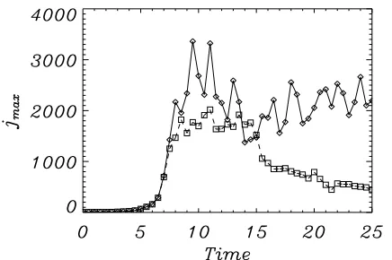
Fig. 3.Maximum current in the domain as a function of time for the experiments withη =0, a grid resolution of 5123 and using driver 1
(solid line and diamonds) and driver 2 (dashed line and squares). The symbols denote each time the current was recorded.
Fig. 4.As for Fig.2at timesa)t=7 andb)t=10, but with driver 2.
seen in Fig.2d. This is then followed by a significant decrease in maximum current as numerical effects cause it to dissipate. However, as the boundaries continue to be driven, the magnetic field continues to be stressed such that at aroundt=17 the cur-rent starts to once again build up. We would expect this process to repeat since the boundaries are continuously driven.
If we now consider the same setup as the above experiment, except that the driver is ramped down aroundt=7 (driver 2) we naturally find a similar behaviour to that shown in Figs.2a−c. Figure3(dashed curve) shows that as the driver starts decreas-ing, the maximum current in the domain increases less rapidly than in the driver 1 case, as one might expect. After t = 7 the maximum current drops but at this time the current in the mid plane for this experiment looks the same as it does for the driver 1 experiment (compare Figs. 4a and 2c). However, by t = 10 the current in the mid-plane of the driver 2 experiment looks quite different to that seen at the same time for driver 1 (compare Figs.4b and2d). The main current layer is still clearly visible and a series of much shorter current sheets are found, but these are not distributed throughout the domain, instead they are clustered around the end of the main current layer forming a bub-ble. The drop offin maximum current that has occurred (Fig.3) suggests that att = 10 numerical reconnection has once again kicked in. The horizontal velocity arrows shown in Fig.5, at this time, indicate that the flow pattern is very similar to that occur-ring in 2D reconnection. There is a fast outflow from the ends of the current sheets, a clear indication that numerical reconnection is occurring. It is possible that fast outflows from this numerical reconnection in the main current sheet, which are heading to-wards each other due to the periodic boundary conditions, lead
Fig. 5.As for Fig.2, but taken at timet=10 withη=0, but witha)
driver 1 andb)driver 2. Arrows show the projected velocity in the plane with the length of the arrows representing the magnitude of the velocity.
to the formation of other short current layers and a disruption of the outflow.
The evolution of the current for both drivers reveals some interesting features which we address in the following sections. Firstly, in Sect. 6, we consider the energetics of the system, to determine whether the current really has dropped due to numer-ical dissipation and to investigate the effects of this for a real physical situation. Secondly, in Sect. 7, we evaluate the three-dimensional nature of the current layer att=7 and the magnetic structure.
6. Energy: total energy and Poynting flux
In order to properly understand the energetics, we consider, in Sect. 6.1, the ideal (η = 0) behaviour, before investigating the effects of uniform resistivity (η=constant) in Sect. 6.2.
First we discuss the total energy equation. Taking appropri-ate combinations of Eqs. (1) to (5), the total energy equation is
∂ ∂t
1 2ρv
2+ p γ−1+
B2 2μ0
+∇·
1 2ρv
2u+ γp γ−1u+
E×B μ0
[image:6.595.323.540.76.514.2] [image:6.595.39.290.278.398.2]
Integrating over the volume of the computational box and using Gauss’s theorem, we have
detot dt +
S
Q·dS=0, (30)
where the total volume integrated energy,etot(t), given by etot(t)=
1 2ρv
2dV+
p γ−1dV+
B2 2μ0
dV, (31)
is the sum of the integrated kinetic energy, internal energy and magnetic energy, respectively and
Q= 1 2ρv
2u+ γp γ−1u+
E×B μ0 ,
(32) is the energy flux into or out of the plasma. Since the side bound-aries are periodic and the top and bottom boundbound-aries havevz=0, the total inflow/outflow of energy is just the Poynting flux, in di-mensionless variables, namely
S
E×B·dS, (33)
whereE=−u×B+ηj. The integral (33) need only be evaluated on the top (z= +L) and bottom (z=−L) boundaries because the sides are periodic. The total energy in the computational box can only increase, in response to the boundary motions, since there is a net flow of Poynting flux into the domain.
6.1. Ideal MHD energetic behaviour (η= 0)
In this section, we restrict our attention to the “ideal” evolu-tion withη =0. This allows us to assess the importance of nu-merical diffusion, which is of course a numerical error, in these simulations.
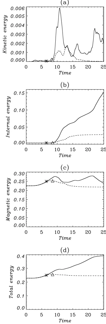
The simulations presented are for runs with a grid resolution of 5123(our maximum resolution). Coarser grids were also run and a similar behaviour was observed. Choosing the highest res-olution for theη = 0 runs ensures there is minimal numerical diffusion of the magnetic field up to aboutt = 7 or 8, after the formation of the current layer. Figure6shows the time evolution of all energies for driver 1 (solid) and driver 2 (dashed). The as-terisk denotes the time (t = 6.5) when the shearing velocity of driver 2 starts to slow down and the triangle corresponds to the time (t=8.5) when it has completely stopped.
For both drivers the magnetic energy dominates over the other energies and is some 50−100 times larger. It is initially al-most constant until aboutt=3 when it begins to rise. Naturally, when driver 2 is ramped down, the energies in the two runs start to differ, with the magnetic energy for driver 1 peaking att=9, whilst, for driver 2, the magnetic energy levels offbetweent=7 and=8.5
[image:7.595.337.520.80.639.2]The kinetic energy for both drivers remains extremely small until the current layer has formed at aroundt=7, when it starts to increase. After a tiny dip the kinetic energy rises rapidly at aroundt = 8.5. This sudden and dramatic increase in kinetic energy is almost certainly due to numerical diffusion causing the magnetic field to reconnect. The rise is more dramatic for driver 1 than driver 2, since driver 1 is continuously driven and so, at the same time that the system is trying to dissipate the strong currents, the driver is continuing to stress the field and so maintain/rebuild the currents. In response to the reconnection, the internal energy begins to rise for both drivers, indicating that the plasma is being heated. Since driver 2 stops att = 8 and,
Fig. 6.Volume integrated energiesa)kinetic,b)internal,c)magnetic, andd)total energy as functions of time forη=0 and driver 1 (solid) and driver 2 (dashed). For the driver 2 experiment, the start (asterisk) of the ramp down and end (triangle) of the ramp down of driver 2 are indicated. These experiments have a grid resolution 5123.
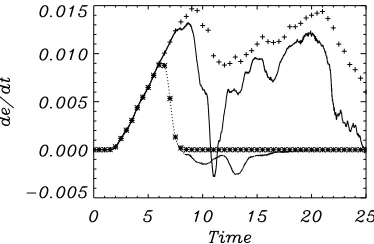
Fig. 7.Instantaneous Poynting flux (driver 1 – plus signs and driver 2 – asterisks) and the rate of change in the total energy, detot/dt, (driver 1
– solid and driver 2 – dotted line) versus time. This experiment was carried out with a grid resolution of 5123.
for driver 2 is once again almost back to zero. The magnetic en-ergy drops offduring this reconnection phase and levels offto an energy slightly below the initial magnetic energy of the numeri-cal run (i.e., to an energy less than that after the first shear of the field). Note, that the final internal energy is only one tenth the final magnetic energy.
For driver 1, on the other hand, the internal energy contin-ues to increase, but at a slightly lower rate, as the Poynting flux continues to add energy into the system which is converted into heat. The kinetic energy in the system is maintained significantly above zero, although at a much lower level than the high peak seen at the start of the numerical diffusion. This suggests that after the rapid onset of reconnection, which results in a drop in magnetic energy, the system adjusts to a quasi-steady state where the injection of magnetic energy, via the Poynting flux, is ap-proximately balanced by the loss of magnetic energy through nu-merical reconnection. Hence, fromt=11 tot=16 the magnetic energy is approximately constant. Att=16, when the magnetic reconnection has essentially abated, the magnetic energy starts to increase again as the continued driving stresses the field as indicated by an increase in current (Fig.3, solid line).
The total energy, as calculated directly by the code, is plotted in Fig.6d. It rises continually in the experiment with driver 1, but decreases aftert=9 for driver 2.
The Poynting flux, as defined in (33), has been calculated numerically and is plotted in Fig.7for each driver, along with the rate of change of total energy (detot/dt) (where etot is de-termined using Eq. (31)) in the plasma. From conservation of energy (Eq. (30)), these two should lie on top of each other, but clearly they do not fort >8. The Poynting flux corresponds to the change in total energy, as plotted in Fig.6d, confirming that the increase in the total energy seen in this figure is due to the energy injected from the boundary driving.
For driver 1, we see that the Poynting flux matches the rate of change in total energy exactly, until a time of aroundt=7. Then the effects of the numerical diffusion become significant and the two curves start to deviate. At a much later time, the two terms seem to approach each other again, before diverging at the end of the experiment. Fromt=7 onwards, when the two curves do not agree, the code is not conserving energy exactly. Clearly, the lack of energy conservation will have consequences. The main concern is with the evolution of the plasma pressure and tem-perature. The changes in magnetic energy should be accounted for by a corresponding change in internal energy (the kinetic en-ergy is much too small to be able to account for these changes), but, since they are not, it is difficult to trust the subsequent evo-lution of the plasma pressure and temperature. This is not just a
consequence of our code, but something that all codes will suffer from. If numerical diffusion occurs, energy is not conserved.
If we now consider the conservation of energy in the experi-ment with driver 2 (Fig.7dotted line and asterisks) we see that the Poynting flux increases, matching the rate of change in en-ergy exactly, until the time at which the driver is switched off: at this time the Poynting flux returns to zero as the driver ceases. However, the rate of change of total energy (as calculated from the individual components) continues to evolve aftert = 8, as does the current layer. So again, the energy budget is not prop-erly accounted for.
The simulations with η = 0 result in the formation of a strong, thin current layer. However, numerical diffusion causes magnetic reconnection and this results in a loss of energy con-servation. We have conducted theseη = 0 experiments as they allow for the best indication of current layer formation, the de-tails of which we consider in the next section. However, since we are also interested in the energetic consequences of the dissi-pation of the current layer, we also conduct a series of constant ηexperiments, as discussed below.
6.2. Resistive MHD energetic behaviour (η= constant)
First, we choose an appropriate constant forη. The value of this uniform physical resistivity needs to be chosen so that it is larger than the numerical diffusion, but is still small. In particular, we aim to pick a value such that the current layers are adequately resolved. This will inevitably reduce the value of the maximum current, as discussed below.
The numerical diffusivity of the code, taking into account the size of our domain and the grid resolution used, is of the order ofvA(Δx)2/2w ≈ 2.3×10⁻⁶, where vA ≈ 1 is the maximum Alfvén speed, 2w≈0.6 is the dynamical length scale andΔx≈ 0.6/512 =1.2×10⁻³is the maximum grid spacing across the current layer (for details seeArber et al. 2007). We select two values forηlarger than this, namely 10−5and 10−4.
In Fig.8, we compare the evolution of the energies from ex-periments using driver 1 and with three different resistivities: η = 0, 10−5 and 10−4. Unfortunately, due to the time step re-strictions and computational resources, it was only possible to run the experiment withη=10−4up to a time oft=15. The ini-tial magnetic energy (Fig.8c) increase is smaller asηincreases. This is due to the fact that the Poynting flux injected into the domain decreases asηincreases (see Fig.10). The Poynting flux depends on the size of the horizontal magnetic field component at the boundaries (as discussed by Galsgaard & Parnell 2005) which changes depending on how the magnetic field evolves (in particular how it is stressed, e.g. whether it reconnects or not). For largerη(more reconnection) these field components are re-duced, leading to a reduction in the amount of energy entering the plasma.
A largerηgives not only more reconnection, but also recon-nection at an earlier time. Both of these factors result in a larger increase in internal energy for largerηdue to the greater Ohmic heating and its earlier onset (Fig.8b).
Fig. 8.Volume integrateda)kinetic,b) internal,c) magnetic, andd)
total energies versus time for experiments with driver 1 and resistivities ofη = 0 (solid),η = 10−5 (dotted) and η = 10−4 (dashed). These
experiments were carried out with a grid resolution of 5123.
[image:9.595.78.255.80.640.2]In all cases, the magnetic reconnection that occurs, whether numerical or associated with the imposedη, converts most of the energy injected by the Poynting flux, and stored as currents by the magnetic field, to internal energy. The kinetic energy changes are really small since only about 10% of total Poynting flux is also converted into kinetic energy (Fig.8a). However, since
Fig. 9.Maximum current magnitude is shown as a function of time for the driver 1 experiments with a 5123grid forη=0 (black, triangles), η = 10−5 (red, squares), andη = 10−4 (blue, crosses). The symbols
[image:9.595.338.525.262.385.2]correspond to the times at which the current is actually recorded in each experiment.
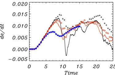
Fig. 10.Poynting flux and the rate of change in the total energy (detot/dt)
are shown as functions of time for experiments using a 5123grid and
driver 1 and resistivityη = 0 (black, plus signs),η =10−5(red,
dia-monds), andη=10−4(blue, asterisks).
the maximum current decreases with increasingη, the magnetic stresses also decrease. Thus, asηincreases, the reconnection be-comes weaker resulting in slower flows and, hence, a smaller maximum kinetic energy.
In Fig.8d we plot the evolution of the total energy for the cases with driver 1, but different values ofη. Not surprisingly, the total energy increases in all cases over time due to the injec-tion of Poynting flux from the boundary driving. However, asη increases the increase in total energy decreases due to the fact that the Poynting flux crossing the boundary is smaller for larger η, as explained above. However, as we see in Fig.8d, at a time of approximatelyt =11 the total energy for theη =10−5case becomes larger than theη=0 case. This does not appear to hap-pen for theη =10−4case and we believe this is due to the fact that we can more accurately follow the flow of energy for this case. This is explained more fully below.
Finally, we look at the conservation of energy for each of these cases (Fig. 10), by plotting the Poynting flux (as calcu-lated by Eq. (33)) and the rate of change of total energy, using Eq. (31). For the experiment withη=10−4the two terms match exactly and for this value ofηwe can correctly follow the flow of energy from the magnetic field to the plasma pressure and tem-perature. Withη =10−5, the two terms are extremely close, al-though there is evidence that numerical diffusion is also present aftert=7, but it is fairly small and does not dominate over our physical magnetic diffusion.
Fig. 11.Isosurface of current at 13% of the maximum current magni-tude at timea)t=7 andb)t=8 for the driver 1 experiment withη=0 and a grid resolution of 5123.
evolution of the system occurs as the numerical diffusion begins to dominate. For the two non-zero values ofη, we are confident that the numerical errors do not dominate and remain small dur-ing the simulations.
7. Current layer structure
We consider the experiment with driver 1 andη =0 and a grid resolution of 5123 at a time of t = 7. As we have discussed above, this experiment has an ideal evolution, with no reconnec-tion, up until approximatelyt=8, unlike the constant non-zero η experiments. Shortly beforet = 7 the maximum current in the experiment shows a sudden very rapid increase. Although the current continues to climb aftert = 7 we pick this time because after this there is evidence of numerical diffusion. We could use either the experiment with driver 1 or driver 2, since both look almost the same, but we choose driver 1 since it has the marginally greater maximum current. Note, that at this stage the plasma pressure and temperature in this experiment should still be correct, since energy conservation still holds as no noticeable numerical diffusion has yet occurred (Fig.10).
Figure11shows isosurfaces of the current magnitude, at ap-proximately 13% of the maximum current in this experiment. Isosurfaces att = 7 andt = 8 are shown in (a) and (b), re-spectively. We clearly see the twisted nature of the current layer. The current layer rotates from bottom to top through an angle of approximately 90◦, since both the first and second shears have approximately equal magnitude. Att = 8 we see that the sheet has started to fragment due to numerical reconnection.
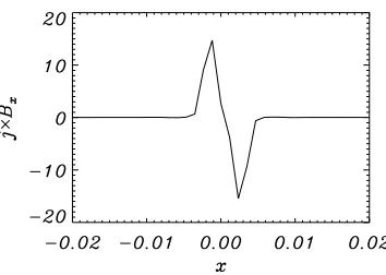
The dominant force is the Lorentz force and itsxcomponent is plotted in Fig.12across the layer (y = 0) at the mid-plane (z = 0). The Lorentz force is zero everywhere except inside the current layer. The width of the nonzero behaviour shown in Fig.12is calculated to be 0.007, which is equivalent to the width of the current layer at this resolution.
7.1. Current layer rotation
[image:10.595.46.284.75.266.2]Figure11shows a gentle rotation of the current layer from the bottom of the box to the top of the box. This rotation appears smooth and, since the plasma is very close to equilibrium when the residual Lorentz forces are analysed, we might expect to
Fig. 12.x-component of the Lorentz force, [j×B]x, across the layer (y=
0) at the mid-plane (z=0-plane) at timet=7. Note, that here−0.02<
x<0.02 to highlight the nonzero behaviour here. The experiment is the driver 1,η=0 case with 5123grid resolution.
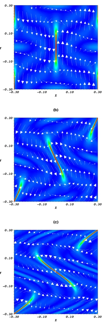
see some form of helical symmetry in the current. Hence, at t = 7, we analyse horizontal slices of the current magnitude atz = 0.0, 0.2 and 0.4 from the middle of the layer working upwards (Fig.13). Due to symmetry the lower section of the current layer is the mirror image of these slices. These slices highlight both the strong currents in the current layers and also show the structure of the weaker current regions in the mid plane. Figure13shows that the current layer twists in an anticlockwise manner for increasingz(for decreasingzit rotates in the clock-wise direction). The layer rotates at an approximately uniform rate with height. The angle of the current layer is approximately −45◦to they-axis atz=0.4, close to the top boundary and ap-proximately half that atz=0.2. The layer is essentially straight in eachzplane but there is a slight bend in the shape at the layer ends due mainly to the imposed periodic boundaries. The ar-rows over plotted denote the vector (Bx,By,0). The field has a squashed elliptical structure near the current layer and there is a clear indication of anti-parallel field on either side of the current layer. The regions of stronger field (i.e. longer arrows) tend to align with the contours of the current magnitude.
The field lines do not cross the current layer. If they did there would be an extremely large Lorentz force. This can be seen in Fig.14which shows field lines plotted in both directions from the mid-plane,z = 0, with starting points along a line−0.2 < y <0.2 that lies either side of the current layer atx=0.01 (red lines) andx=−0.01 (green lines). It is clear that the field lines lie along the current layer, following the same twisted structure as the isosurface of the current. In addition, it is obvious that the green and red field lines are at a different angle to each other. This is expected since the field lines lie on either side of the current layer.
We now investigate the rotation of the current layer by deter-mining the straight line that the layer lies along at each heightz. The current layer passes throughx= 0 andy=0 for allzand so we choose a value foryand determine the value ofx=xmax, wherexmax is the location of the maximum current. Then, we usey/xmax = tanθ(z), to calculate θ(z), the angle between the current layer and thexaxis.θ=π/2 corresponds to the current layer lying along theyaxis. Figure15shows howθvaries with zas we move up the current layer fromz=−0.5 toz=0.5 for y=0.05. Apart from the regions near the boundaries, the twist appears linear in height.
7.2. Magnetic structure
Fig. 13.Slices of the current magnitude in horizontal planesa)z=0,b) z=0.2, andc)z=0.4. The arrows denote the vector [Bx,By,0] in the planes. The experiment is the driver 1,η=0 case with a grid resolution of 5123. Red corresponds to a maximum of 100 while blue corresponds
to a minimum value of 0.
clear that there is a rapid change in the component of the mag-netic field parallel to the current layer,By, across the layer and that the perpendicular component,Bx, is essentially zero. Since
jz = ∂ By ∂x −
∂Bx
[image:11.595.85.260.86.627.2]∂y and, ∂∂yBx is essentially negligible, we expect the jump in By (1.62) to be approximately equal to jzdx (1.61) which it is. Hence, we are satisfied that the magnetic field’s
Fig. 14.Magnetic fieldlines drawn from starting points along the line
−0.2 < y <0.2 atz =0, x=0.01 (red lines) andx =−0.01 (green
lines) att=7 taken from the experiment using driver 1,η=0 and 5123
[image:11.595.350.517.315.434.2]resolution.
Fig. 15.Current layer angle as a function ofzusing y = 0.05. This is taken att =7 with the experiment using driver 1,η=0 and 5123
resolution.
behaviour is consistent with the behaviour of the current.Bz ap-pears to have a rapid rise inside the current layer. This is to be ex-pected. The total pressure, i.e. the magnetic and plasma pressure, across the current layer must be continuous and this is clearly seen in Fig.16c. The gas pressure remains small compared to the magnetic pressure. Therefore, asByvanishes at the centre of the current layer,Bz must increase rapidly at the centre of the layer to ensure that total pressure is continuous.
We have generated a twisted current layer and the only loca-tion so far assessed is thez=0 plane, where the layer is straight and lying along theyaxis. Moving away fromz = 0, the an-gle of the current layer changes and we must calculate magnetic field components along a cut perpendicular to the current layer at various heights. The orientation of the current layer at various values ofzis determined and a cut perpendicular to the current layer atz=0.2 is analysed here. In Fig.17a we plot the normal and tangential components ofBatz = 0.2. Here, as expected, the normal component is much smaller than the tangential. We also see in Fig.17b that the total pressure perpendicular to the layer atz=0.2 is similar to that atz=0.
Fig. 16.Magnetic field components plotted att = 7 across the layer (y=0) at the mid-plane.a)ShowsBx(dashed line) andBy(solid line),
b)showsBz, andc)shows the total pressure (p+B
2
2μ). These are taken att=7 with the experiment using driver 1,η=0 and 5123resolution.
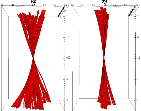
line straighten out. Hence, as expected, when boundary driving stops, the magnetic field lines start to untangle and relax back towards a lower energy state.
However, for driver 1, when the shearing motion is contin-ued, the field lines remain sheared and the isosurface of current still shows a fragmented current layer. Once the current layer forms and reconnection starts, the internal energy continues to rise (as shown in Fig.6) as the Poynting flux crossing the bound-aries is continually dissipated as heat.
7.3. Plasma response
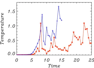
[image:12.595.346.524.78.356.2]Figure19shows how the temperature atx=y =z =0 varies, for theη = 10−5 andη = 10−4experiments with driver 1, as a function of time. Initially the temperature is only 0.00667. What is clear is that the temperature remains low, in both cases, until the current layer forms aroundt = 7 and strong reconnection begins. Forη=10−5, the temperature rises to around 1.0, which
Fig. 17.a)Normal (B⊥) and tangential (B) components ofBacross and along the current layer are plotted in thez =0-plane (solid lines) and thez = 0.2-plane (dashed lines). Obviously, the components that show a sudden switch in sign are theB⊥components.b)Total pressure perpendicular to the current layer in thez=0-plane (solid line) and the
[image:12.595.313.550.448.635.2]z=0.2-plane (dashed line). These are taken att=7 for the experiment using driver 1,η=0 and 5123resolution.
Fig. 18.Magnetic fieldlines drawn from starting points along a line
−0.2< y <0.2 atx=0,z=0 at a timet=25 for the experiments with
η=0 and grid resolution 5123anda)driver 1 andb)driver 2.
Fig. 19.Temperature at x = y = z = 0 as a function of time for the experiment using driver 1, a grid resolution of 5123and withη=10−5
(red, asterisks) andη=10−4(blue, plus signs).
t = 14. Obviously, the larger value of η increases the Ohmic heating term and increases the temperature at the expense of the magnetic energy (see Fig.8). The temperature response of the plasma will be investigated in more detail in future work. It is suffice to state that the temperature can easily reach the required coronal values.
8. Conclusions and future work
In this paper, we have performed a series of numerical exper-iments to investigate in more detail the formation of current layers. The initial field was sheared analytically in thex direc-tion, which was justified when numerical simulations showed agreement with the analytical form used. A second, perpendicu-lar shear was then imposed numerically through photospheric boundary motions. A choice of two different photospheric drivers were used for the second shear. While both shearing ve-locities are gradually ramped up to a constant value, one remains steady thereafter, while the other is ramped down to zero once the strong current layer has formed. Until the current layer for-mation, the magnetic energy dominates both the kinetic energy and the internal energy. The magnetic energy rises due to the stresses injected through the boundary motions. There are dif-ferences only after the twisted current structure has formed.
While theη=0 experiment does produce the largest current values, total energy is not conserved once numerical reconnec-tion begins. Hence, caureconnec-tion must be taken when following the ideal evolution. For a nanoflare model for coronal heating this is a problem, since it is not possible to account for all the energy released when the magnetic energy is reduced. The main error is in the calculation of the internal energy and, hence, the temper-ature and pressure. Non-zero values ofη were also considered and it was shown that the total energy was indeed conserved throughout the simulations. So although physically too large, we can correctly follow the flow of energy into heat.
The current structure is twisted at a uniform rate with height. The projection of the magnetic field onto azplane shows that the field lines are essentially elliptical in nature. The regions of strong field tend to align with the contours of the current mag-nitude, as one would expect. Examining the current components we findjzto be dominant, which agrees with previous numerical studies, for exampleGalsgaard & Nordlund(1996b).
Before the current layer forms, the boundary motions gen-erate a Poynting flux that results in an increase in the magnetic energy. It is only after the strong currents form and reconnec-tion starts, that this magnetic energy is released. A continued
driving of the photospheric boundary, as for driver 1, means that Poynting flux continues to be fed into the system and is almost immediately converted into internal energy and, hence, temperature. Thus, if there are current layers already present in the corona, any photospheric motions that increase the stresses (currents) in the field, could produce heating. In the absence of current layers, the motions result in an increase of magnetic en-ergy and the possible formation of current layers, but no sig-nificant heating. This is in agreement with the results found by Rappazzo & Parker(2013) who show that an initial configura-tion with a large-scale magnetic field develops small scales only above a magnetic intensity threshold.
Isosurfaces of temperature show that its maximum value oc-curs around the central plane at z = ±0.15. The temperature at the centre of the simulation reaches a dimensionless value between 1.1 and 1.4, depending on the value of η. Although this value is quite localised, thermal conduction will spread the temperature along the field lines, reducing the maximum value. Further work is needed to understand the thermodynamic impli-cations in detail. Using the typical values of Sect.2.1, namely B0 =10 G,ne=5×10¹⁴m−3 andL0 =50 Mm, the velocities are scaled byv0=975.5 km s−1, the time is in units oft0=51 s and the temperature in units ofT0 = 5.7×10⁷ K. The maxi-mum temperature is about 6×10⁷K forη=10−5and the rapid heating due to the rapid release of magnetic energy occurs over nearly 2 time units or 100 s. It is slightly higher whenηis larger. This temperature is high but is consistent with the temperatures found byHood et al.(2009), when considering heating by Taylor relaxation.Botha et al.(2011) showed that these high localized temperatures were reduced by a factor of 10 and spread out along the field when thermal conduction, parallel to the magnetic field, is included.
These illustrative temperatures depend on the choice of background parameters. Considering a stronger magnetic region, withB0 =50 G, slightly denser plasma,ne =1015m−3, but the same length forL0, we find that the maximum temperature is now around 8×10⁸K forη=10−5and the rapid rise in temper-ature occurs within only 30 s.
There various extensions to this work that will be presented in future articles.
1. Once the photospheric driving is switched off, the magnetic field tries to relax towards its lowest energy state. Since, the boundary motions have injected helicity into the plasma, the final state should be a linear force-free field with the same magnetic helicity as that at the time the driving is stopped. 2. A detailed study into the reconnection process could be
un-dertaken. There are no null points in the magnetic field and so the reconnection may be due to quasi-separator reconnec-tion. However, this must be checked by investigating the par-allel component of the electric field to see where the recon-nection is occurring.
3. There is some evidence that the current layer starts to frag-ment once reconnection begins. It is likely that there is a turbulent cascade to smaller and smaller current structures. Thus, a comparison with the work ofRappazzo et al.(2007, 2008) should be carried out.
4. The inclusion of parallel thermal conduction and optically thin radiation will provide predictions of the temperature and, using forward modelling techniques, we can compare with observed properties of coronal loops.
Acknowledgements. The simulations were run on the UK MHD cluster at the
University of St. Andrews funded by STFC/SRIF. R. Bowness acknowledges
References
Al-Hachami, A. K., & Pontin, D. I. 2010, A&A, 512, A84
Arber, T. D., Longbottom, A. W., Gerrard, C. L., & Milne, A. M. 2001, J. Comput. Phys., 171, 151
Arber, T. D., Haynes, M., & Leake, J. E. 2007, ApJ, 666, 541
Aulanier, G., Pariat, E., Démoulin, P., & DeVore, C. R. 2006, Sol. Phys., 238, 347
Bhattacharyya, R., Low, B. C., & Smolarkiewicz, P. K. 2010, Phys. Plasmas, 17, 112901
Botha, G. J. J., Arber, T. D., & Hood, A. W. 2011, A&A, 525, A96 Browning, P. K., & Hood, A. W. 1989, Sol. Phys., 124, 271
Browning, P. K., Gerrard, C., Hood, A. W., Kevis, R., & van der Linden, R. A. M. 2008, A&A, 485, 837
Bungey, T. N., & Priest, E. R. 1995, A&A, 293, 215 Cargill, P. J. 1993, Sol. Phys., 147, 263
Cargill, P. J., & Klimchuk, J. A. 1997, ApJ, 478, 799 Cargill, P. J., & Klimchuk, J. A. 2004, ApJ, 605, 911
Craig, I. J. D., & Litvinenko, Y. E. 2005, Phys. Plasmas, 12, 032301
Dahlburg, R. B., Einaudi, G., Rappazzo, A. F., & Velli, M. 2012, A&A, 544, L20 De Moortel, I., & Galsgaard, K. 2006a, A&A, 451, 1101
De Moortel, I., & Galsgaard, K. 2006b, A&A, 459, 627
Démoulin, P., Priest, E. R., & Lonie, D. P. 1996, J. Geophys. Res., 101, 7631 Fuentes-Fernández, J., & Parnell, C. E. 2012, A&A, 544, A77
Fuentes-Fernández, J., & Parnell, C. E. 2013, A&A, 554, A145
Fuentes-Fernández, J., Parnell, C. E., & Hood, A. W. 2011, A&A, 536, A32 Galsgaard, K., & Nordlund, Å. 1996a, J. Geophys. Res., 101, 13445 Galsgaard, K., & Nordlund, Å. 1996b, J. Geophys. Res., 101, 13445 Galsgaard, K., & Parnell, C. E. 2005, A&A, 439, 335
Green, R. M. 1965, in Stellar and Solar Magnetic Fields, ed. R. Lust, IAU Symp., 22, 398
Gudiksen, B. V., & Nordlund, A. 2006, in 36th COSPAR Scientific Assembly, COSPAR, Plenary Meeting, 36, 3545
Haynes, A. L., Parnell, C. E., Galsgaard, K., & Priest, E. R. 2007, Roy. Soc. London Proc. Ser. A, 463, 1097
Hood, A. W., Browning, P. K., & van der Linden, R. A. M. 2009, A&A, 506, 913 Huang, Y.-M., Bhattacharjee, A., & Zweibel, E. G. 2010, Phys. Plasmas, 17,
055707
Janse, Å. M., & Low, B. C. 2009, ApJ, 690, 1089
Klimchuk, J. A., & Cargill, P. J. 2001, ApJ, 553, 440 Krucker, S., & Benz, A. O. 2000, Sol. Phys., 191, 341 Lau, Y.-T., & Finn, J. M. 1990, ApJ, 350, 672 Levine, R. H. 1974, ApJ, 190, 457
Longbottom, A. W., Rickard, G. J., Craig, I. J. D., & Sneyd, A. D. 1998, ApJ, 500, 471
Longcope, D. W., & Cowley, S. C. 1996, Phys. Plasmas, 3, 2885 Lothian, R. M., & Hood, A. W. 1989, Sol. Phys., 122, 227
Masson, S., Pariat, E., Aulanier, G., & Schrijver, C. J. 2009, ApJ, 700, 559 Mellor, C., Gerrard, C. L., Galsgaard, K., Hood, A. W., & Priest, E. R. 2005, Sol.
Phys., 227, 39
Parker, E. N. 1972, ApJ, 174, 499 Parker, E. N. 1987, Sol. Phys., 111, 297 Parker, E. N. 1988, ApJ, 330, 474
Parnell, C. E., & Jupp, P. E. 2000, ApJ, 529, 554
Parnell, C. E., DeForest, C. E., Hagenaar, H. J., et al. 2009, ApJ, 698, 75 Parnell, C. E., Maclean, R. C., & Haynes, A. L. 2010a, ApJ, 725, L214 Parnell, C. E., Maclean, R. C., & Haynes, A. L. 2010b, ApJ, 725, L214 Pontin, D. I., & Craig, I. J. D. 2005, Phys. Plasmas, 12, 072112
Pontin, D. I., Bhattacharjee, A., & Galsgaard, K. 2007a, Phys. Plasmas, 14, 052106
Pontin, D. I., Bhattacharjee, A., & Galsgaard, K. 2007b, Phys. Plasmas, 14, 052109
Priest, E. R., & Démoulin, P. 1995, J. Geophys. Res., 100, 23443 Priest, E. R., & Pontin, D. I. 2009, Phys. Plasmas, 16, 122101 Priest, E. R., Longcope, D. W., & Heyvaerts, J. 2005, ApJ, 624, 1057 Rappazzo, A. F., & Parker, E. N. 2013, ApJ, 773, L2
Rappazzo, A. F., Velli, M., Einaudi, G., & Dahlburg, R. B. 2007, ApJ, 657, L47 Rappazzo, A. F., Velli, M., Einaudi, G., & Dahlburg, R. B. 2008, ApJ, 677, 1348 Rappazzo, A. F., Velli, M., & Einaudi, G. 2010, ApJ, 722, 65
Rickard, G. J., & Titov, V. S. 1996, ApJ, 472, 840
Schrijver, C. J., & Zwaan, C. 2000, Solar and Stellar Magnetic Activity (New York: Cambridge University Press), 34
Schrijver, C. J., Title, A. M., van Ballegooijen, A. A. ., Hagenaar, H. J., & Shine, R. A. 1997, ApJ, 487, 424
Syrovatskiˇı, S. I. 1971, Sov. J. Exp. Theor. Phys., 33, 933 van Leer, B. 1979, J. Comput. Phys., 32, 101